k-近邻(kNN)算法是一种非常简单有效的监督学习算法,该算法根据测试样本和训练样本之间的距离(在特征所构成的高维空间),对测试样本进行分类。简单地说,kNN采用的是“近朱者赤近墨者黑”的思想。
基本原理及算法
- 输入的样本集中,每个数据都存在标签
- 输入没有标签的新数据后,对比新数据的每个特征和样本集中每个样本对应的特征
- 提取样本集中特征最相近的k个数据所对应的标签
- 选择这k个标签中出现次数最多的分类,作为新数据的分类
1 | from numpy import * |
测试算法
生成数据集
1 | def creatDataSet(): |
1 | group, labels = creatDataSet() |
[[ 1.   1.1]
 [ 1.   1. ]
 [ 0.   0. ]
 [ 0.   0.1]]
['A', 'A', 'B', 'B']
测试算法
1 | classfy0([0, 0], group, labels, 3) |
'B'实例1:改进约会网站
数据准备
1 | def file2matrix(filename): |
1 | datingDataMat, datingLables = file2matrix(r'/media/seisinv/Data/course/ai/machine_learning_in_action/Machine-learning-in-action/k-Nearest Neighbor/datingTestSet2.txt') |
[[  4.09200000e+04   8.32697600e+00   9.53952000e-01]
 [  1.44880000e+04   7.15346900e+00   1.67390400e+00]
 [  2.60520000e+04   1.44187100e+00   8.05124000e-01]
 ...,
 [  2.65750000e+04   1.06501020e+01   8.66627000e-01]
 [  4.81110000e+04   9.13452800e+00   7.28045000e-01]
 [  4.37570000e+04   7.88260100e+00   1.33244600e+00]]
[3, 2, 1, 1, 1, 1, 3, 3, 1, 3, 1, 1, 2, 1, 1, 1, 1, 1, 2, 3]
数据可视化
1 | import matplotlib |
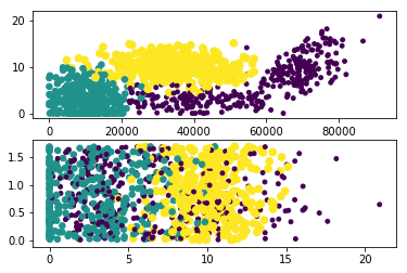
数据可视化
数据预处理
1 | def autoNorm(dataSet): |
1 | normMat, ranges, minValues = autoNorm(datingDataMat) |
[[ 0.44832535  0.39805139  0.56233353]
 [ 0.15873259  0.34195467  0.98724416]
 [ 0.28542943  0.06892523  0.47449629]
 ...,
 [ 0.29115949  0.50910294  0.51079493]
 [ 0.52711097  0.43665451  0.4290048 ]
 [ 0.47940793  0.3768091   0.78571804]]
[[  9.12730000e+04   2.09193490e+01   1.69436100e+00]]
[[ 0.        0.        0.001156]]
验证算法
使用90%的数据用来作为训练数据(尽管kNN不需要训练过程),10%的数据用来测试算法性能
1 | def datingClassTest(): |
1 | datingClassTest() |
The classifier came back with: 3, the real answer is: 3
The total error rate is: 0.050000
测试算法
终端输入用户信息,作为测试数据,判断约会情况
1 | def classifyPerson(): |
1 | classifyPerson() |
percentage of time spent playing video game?10
frequency flier miles earned per year?10000
liters of ice cream consumed per year?0.5
You will probably like this person:  in small doses
实例2 手写识别系统
数据预处理
1 | def img2vector(filename): |
验证算法
1 | from os import * |
1 | handwriteClassTest() |
the classifier came back with: 4, the real number is: 4
the classifier came back with: 1, the real number is: 1
the classifier came back with: 2, the real number is: 2
the classifier came back with: 3, the real number is: 3
the classifier came back with: 4, the real number is: 4
the classifier came back with: 5, the real number is: 5
the classifier came back with: 6, the real number is: 6
the classifier came back with: 7, the real number is: 7
the classifier came back with: 8, the real number is: 8
the classifier came back with: 9, the real number is: 9

 the total number of errors is: 12

 the total error rate is: 0.012685
使用算法
可以使用自己手写的数据输入
结论及讨论
结论
kNN算法简单有效,有以下特点:
> + 优点:精度高、对异常值不敏感、无数据输入假设
> + 缺点:计算复杂度高(需要计算每个输入样本和训练样本集中所有样本的距离),空间复杂度高(需要存储所有的训练样本数据)
讨论
周志华在《机器学习》一书对kNN的点评: > + kNN虽然简单,但是它的泛化错误率不超过贝叶斯最优分类器错误率的2倍
> + 上述结论的前提是测试样本附近任意小的距离内总能找到一个训练样本,当属性维度为20时,每个维度要求\(10^3\),则一共需要\(10^60\)个样本。实际情况往往成千上万个属性,要满足密度采样条件所需要的样本是无法达到的天文数字。另外,计算这么多样本与测试样本之间的距离,也不容易。实际上,在高维情况下出现的样本稀疏、距离计算困难,是所有机器学习算法共同面临的严重障碍,被称为“维数灾难”(curse of dimensionality)。
参考资料
- Peter Harrington, Machine learning in action, Manning Publications, 2012
- 周志华,机器学习,清华大学出版社, 2016