决策树是一种非常常用的数据挖掘算法。以分类问题为例,它根据一系列子问题形成树结构进行决策,这也是人类在面临决策问题时一种很自然的处理机制,因此是也是知识图谱的重要算法之一。该算法采用的是分而治之(divide-and-conquer)的思想。本文主要介绍决策树中的ID3算法。
基本原理及算法
香农熵/信息熵
信息熵(information entropy)是度量样本集合纯度最常用的一个指标,假定当前样本集合\(D\)中第\(k\)类样本所占的比例为\(p_k\)(k=1,2,...,K),则\(D\)的信息熵定义为: \[Ent(D) = - \sum_{k=1}^{K} p_k log_2{p_k}\] Ent(D)的值越小,样本集合\(D\)的纯度越高。
1 | from math import log |
1 | def createDataSet(): |
1 | myData, labels = createDataSet() |
1 | myData |
[[1, 1, 'yes'], [1, 1, 'yes'], [1, 0, 'no'], [0, 1, 'no'], [0, 1, 'no']]1 | calcShannonEnt(myData) |
0.97095059445466861 | # 正概率和负概率组合 |
0.97095059445466861 | # 增加一种类别 |
[[1, 1, 'maybe'], [1, 1, 'yes'], [1, 0, 'no'], [0, 1, 'no'], [0, 1, 'no']]熵越高,数据的纯度越低
1 | calcShannonEnt(myData) # 熵越高,数据的纯度越低 |
1.3709505944546687划分数据集
信息增益用来衡量用属性\(a\)划分数据集所获得的“纯度提升”。信息增益越大,“纯度提升”越大。
假定离散属性\(a\)有\(V\)个可能的取值\({a^1, a^2, ..., a^V}\),若使用属性\(a\)来对样本集\(D\)进行划分,则会产生\(V\)个分支节点,其中第\(v\)个分支包含了属性\(a\)取值为\(a^v\)的样本集合\(D^v\)。根据信息熵的定义,可以计算样本集合\(D^v\)的信息熵。再考虑到不同的分支节点所包含的样本数不同,给各个分支节点取权重\(|D|^v/|D|\),即样本数越多的分支节点的影响越大,因此可以计算出用属性\(a\)对样本进行划分所获得的“信息增益”: \[Gain(D, a) = Ent(D) - \sum_{v=1}^{V} \frac{|D^v|}{|D|}Ent(D^v)\] 划分数据集所选择的属性应当满足: \[a_* = arg max_{a \in A} Gain(D, a)\] 使得每个分支节点的数据集熵\(Ent(D^v)\)最小化(纯度最大化)。
1 | def splitDataSet(dataSet, axis, value): |
1 | myDat, labels = createDataSet() |
[[1, 1, 'yes'], [1, 1, 'yes'], [1, 0, 'no'], [0, 1, 'no'], [0, 1, 'no']]1 | splitDataSet(myDat, 0, 1) |
[[1, 'yes'], [1, 'yes'], [0, 'no']]1 | splitDataSet(myDat, 0, 0) |
[[1, 'no'], [1, 'no']]1 | def choosBestFeatureTopSplit(dataSet): |
1 | choosBestFeatureTopSplit(myDat) |
0递归构建决策树
工作原理: 1. 输入原始数据集 2. 根据信息增益最大化准则选择最优属性 3. 根据最优属性划分数据集 4. 第一次划分之后再次划分
递归终止条件: 1. 遍历所有属性 2. 每个分支下的所有样本属于同一类
1 | import operator |
1 | def createTree(dataSet, labels): |
1 | myDat, labels = createDataSet() |
{'no surfacing': {0: 'no', 1: {'flippers': {0: 'no', 1: 'yes'}}}}绘制树形图
和kNN不同,决策树算法的数据形式含义十分清晰,可以借助画图工具将其绘制出来。
1 | def getNumLeafs(myTree): |
1 | print(getNumLeafs(myTree)) |
3
2
1 | a = list(myTree.keys())[0] |
{0: 'no', 1: {'flippers': {0: 'no', 1: 'yes'}}}1 | import matplotlib.pyplot as plt |
1 | createPlot(myTree) |
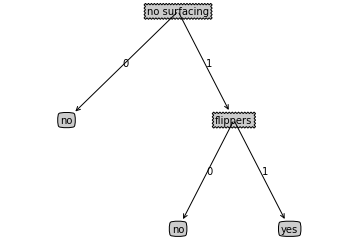
简单的树形图
使用决策树进行分类
1 | def classify(inputTree, featLabels, testVec): |
1 | def retrieveTree(i): |
1 | myDat, labels = createDataSet() |
'no'1 | classify(myTree, labels, [1, 1]) |
'yes'使用算法
构造决策树十分耗时,解决方案是把决策树存在磁盘中,使用时调用即可。
1 | def storeTree(inputTree, filename): |
1 | storeTree(myTree, 'classifier_dt.txt') |
{'no surfacing': {0: 'no', 1: {'flippers': {0: 'no', 1: 'yes'}}}}1 | myTree |
{'no surfacing': {0: 'no', 1: {'flippers': {0: 'no', 1: 'yes'}}}}实例:预测隐形眼镜类型
1 | fr = open('lenses.txt') |
1 | lensesTree |
{'tearRate': {'normal': {'astigmatic': {'no': {'age': {'pre': 'soft',
      'presbyopic': {'prescript': {'hyper': 'soft', 'myope': 'no lenses'}},
      'young': 'soft'}},
    'yes': {'prescript': {'hyper': {'age': {'pre': 'no lenses',
        'presbyopic': 'no lenses',
        'young': 'hard'}},
      'myope': 'hard'}}}},
  'reduced': 'no lenses'}}
1 | createPlot(lensesTree) |
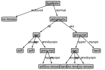
构建的决策树
结论及讨论
结论
优点:计算复杂度不高,输出结果容易理解,对中间值缺失不敏感,可以处理不相关特征数据
缺点:可能会产生过拟合,此时需要裁剪决策树
讨论
- 对过拟合问题,可以采用剪枝,包括预剪枝和后剪枝。预剪枝是指在决策树生成过程中,对每个节点在划分前后进行估计,若当前节点的划分不能带来决策树泛化性能提升,则停止划分,并将当前节点记为叶节点;后剪枝则是先从训练集生成一颗完整的决策树,然后自底而上地对非叶节点进行考察,若将该节点对应的子树替换为叶节点也能带来决策树泛化性能提升,则将该子树替换为叶节点。
- 对连续属性,最简单的策略是采用二分法进行处理。对不同的候选划分点,采用和属性优选相同的策略,选出最优的划分点对该连续属性进行划分。
- 缺失值处理,需要回答两个问题:(1)如何选择属性?(2)给定划分属性,如何划分?首先对根节点的各个样本设置权值为1,在构建决策树的过程中,更新各个样本的权值。问题(1)的解决方案是对无缺失值的样本集计算信息增益,然后乘以无缺失值所占的比例,得到修正后的信息增益,再根据信息增益最大化选择属性;对于问题(2),如果样本在划分属性上的值已知,则将该样本划入与该值对应的子节点,并保持该样本的样本权值,如果样本在划分属性上值未知,则将该样本划入所有的子节点,但是该样本的样本权值调整为原来的权值乘以无缺失样本占该属性上取某值的样本所占的比例,这样就让同一个(缺失值)样本以不同的概率划入到不同的子节点中去。
- 多变量决策树,前面讨论的决策树形成的分类边界有一个明显的特征:轴平行,当学习任务的真实分类边界比较复杂时,必须使用很多段划分才能得到较好的近似,此时的决策树会相当复杂。原来的非叶节点是针对某个属性划分,改成对属性的线性组合进行测试,从而使得学习过程从对每个非叶节点寻找最优属性,变为建立一个合适的线性分类器。
参考资料
- Peter Harrington, Machine learning in action, Manning Publications, 2012
- 周志华,机器学习,清华大学出版社, 2016