逻辑回归可以看做只有输入和输出层的神经网络,本文介绍单个隐藏层的神经网络,并应用其进行二分类,利用非线性激活函数对线性不可分数据进行预测。涉及包括非线性激活函数的种类和功能、隐藏层的作用、梯度的计算等内容。
数据加载
1 | # Package imports |
1 | X, Y = load_planar_dataset() |
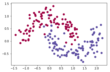
1 | # Visualize the data: |
png
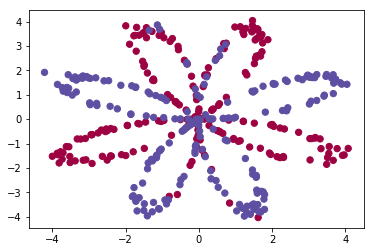
数据包括:
- 矩阵X,每个样本包含两个特征(x1, x2)
- 向量Y,每个样本取值0/1(红色:0, 蓝色:1).
1 | ### START CODE HERE ### (≈ 3 lines of code) |
The shape of X is: (2, 400)
The shape of Y is: (1, 400)
I have m = 400 training examples!
逻辑回归
为了对比逻辑回归的效果,采用sklearn自带的逻辑回归算法进行测试
1 | # Train the logistic regression classifier |
/home/seisinv/anaconda3/envs/tensorflow/lib/python3.5/site-packages/sklearn/utils/validation.py:547: DataConversionWarning: A column-vector y was passed when a 1d array was expected. Please change the shape of y to (n_samples, ), for example using ravel().
  y = column_or_1d(y, warn=True)
1 | # Plot the decision boundary for logistic regression |
Accuracy of logistic regression: 47 % (percentage of correctly labelled datapoints)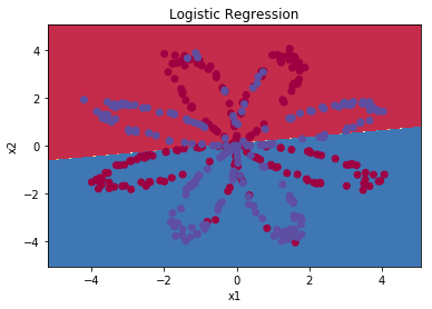
png
小结:由于数据不是线性可分的,所以逻辑回归表现不好。
神经网络模型
模型图: 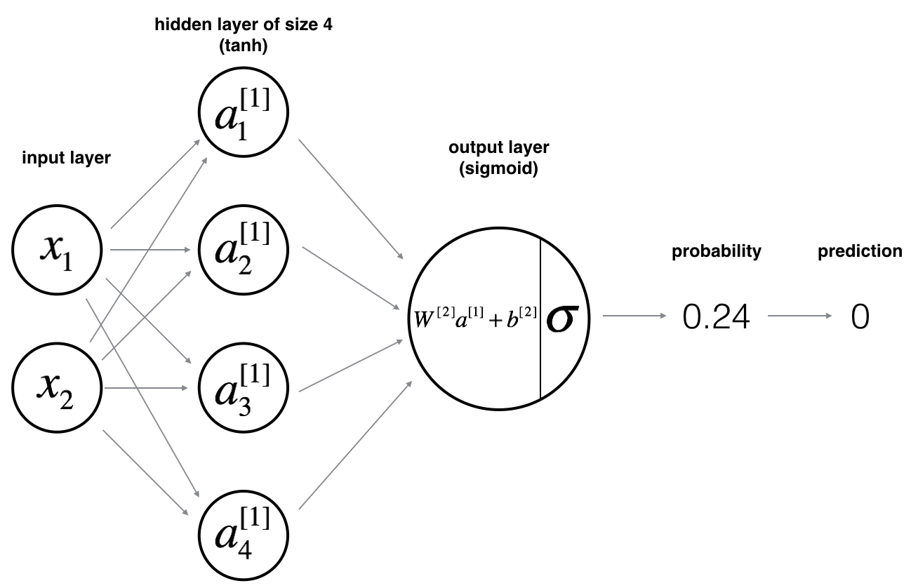
数学公式:
对一个样本 \(x^{(i)}\): \[z^{[1] (i)} = W^{[1]} x^{(i)} + b^{[1] (i)}\tag{1}\] \[a^{[1] (i)} = \tanh(z^{[1] (i)})\tag{2}\] \[z^{[2] (i)} = W^{[2]} a^{[1] (i)} + b^{[2] (i)}\tag{3}\] \[\hat{y}^{(i)} = a^{[2] (i)} = \sigma(z^{ [2] (i)})\tag{4}\] \[y^{(i)}_{prediction} = \begin{cases} 1 & \mbox{if } a^{[2](i)} > 0.5 \\ 0 & \mbox{otherwise } \end{cases}\tag{5}\]
给定所有样本的预测值,计算代价函数 \(J\) : \[J = - \frac{1}{m} \sum\limits_{i = 0}^{m} \large\left(\small y^{(i)}\log\left(a^{[2] (i)}\right) + (1-y^{(i)})\log\left(1- a^{[2] (i)}\right) \large \right) \small \tag{6}\]
流程: 1. 定义神经网络结构 ( 输入单元个数、隐藏层神经元个数等). 2. 模型参数初始化 3. 循环: - 正向传播 - 计算损失函数 - 反传计算梯度 - 更新参数(梯度下降法)
定义神经网络结构
对于单隐藏层神经网络,关于神经网络结构有三个超参: - n_x: 输入层大小 - n_h: 隐藏层大小 (本文定义为4) - n_y: 输出层大小
1 | # GRADED FUNCTION: layer_sizes |
1 | X_assess, Y_assess = layer_sizes_test_case() |
The size of the input layer is: n_x = 5
The size of the hidden layer is: n_h = 4
The size of the output layer is: n_y = 2
初始化模型参数
利用随机函数初始化模型参数w,零初始化b。
1 | # GRADED FUNCTION: initialize_parameters |
1 | n_x, n_h, n_y = initialize_parameters_test_case() |
W1 = [[-0.00416758 -0.00056267]
 [-0.02136196  0.01640271]
 [-0.01793436 -0.00841747]
 [ 0.00502881 -0.01245288]]
b1 = [[ 0.]
 [ 0.]
 [ 0.]
 [ 0.]]
W2 = [[-0.01057952 -0.00909008  0.00551454  0.02292208]]
b2 = [[ 0.]]
循环迭代
- 激活函数既可以采用sigmoid函数(已经实现)和tanh函数(np.tanh());
- 具体步骤包括:
- 从字典"parameters"中读取参数
- 正传,计算 \(Z^{[1]}, A^{[1]}, Z^{[2]}\) and \(A^{[2]}\)
- 从字典"parameters"中读取参数
- 反传中需要的变量都存在"
cache"中
1 | # GRADED FUNCTION: forward_propagation |
1 | X_assess, parameters = forward_propagation_test_case() |
-0.000499755777742 -0.000496963353232 0.000438187450959 0.500109546852计算好了\(A^{[2]}\) (Python 变量为 "A2"), 它包含了每个样本\(a^{[2](i)}\) , 那么可以根据下面的公式计算代价函数: \[J = - \frac{1}{m} \sum\limits_{i = 0}^{m} \large{(} \small y^{(i)}\log\left(a^{[2] (i)}\right) + (1-y^{(i)})\log\left(1- a^{[2] (i)}\right) \large{)} \small\tag{13}\]
1 | # GRADED FUNCTION: compute_cost |
1 | A2, Y_assess, parameters = compute_cost_test_case() |
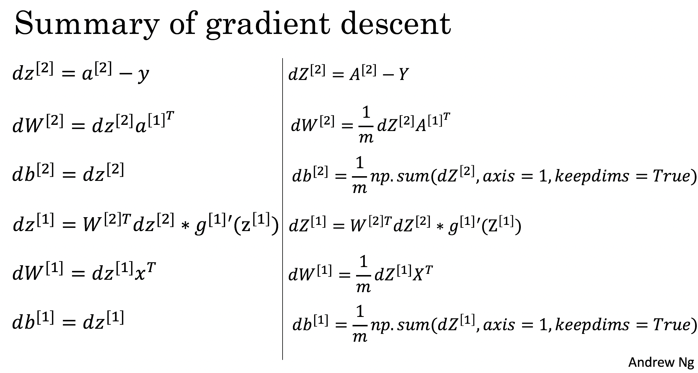
cost = 0.692919893776反传是神经网络中(数学上)最复杂的一步:
1 | # GRADED FUNCTION: backward_propagation |
1 | parameters, cache, X_assess, Y_assess = backward_propagation_test_case() |
dW1 = [[ 0.01018708 -0.00708701]
 [ 0.00873447 -0.0060768 ]
 [-0.00530847  0.00369379]
 [-0.02206365  0.01535126]]
db1 = [[-0.00069728]
 [-0.00060606]
 [ 0.000364  ]
 [ 0.00151207]]
dW2 = [[ 0.00363613  0.03153604  0.01162914 -0.01318316]]
db2 = [[ 0.06589489]]梯度下降法准则:$ = - $,其中 \(\alpha\) 是学习率, \(\theta\) 代表待求的参数.
当学习率合理时,梯度下降法收敛;当学习率太小,收敛太慢;当学习率太大,容易发散。下面的图来自Adam Harley。
1 | # GRADED FUNCTION: update_parameters |
1 | parameters, grads = update_parameters_test_case() |
W1 = [[-0.00643025  0.01936718]
 [-0.02410458  0.03978052]
 [-0.01653973 -0.02096177]
 [ 0.01046864 -0.05990141]]
b1 = [[ -1.02420756e-06]
 [  1.27373948e-05]
 [  8.32996807e-07]
 [ -3.20136836e-06]]
W2 = [[-0.01041081 -0.04463285  0.01758031  0.04747113]]
b2 = [[ 0.00010457]]
整合成神经网络模型
1 | # GRADED FUNCTION: nn_model |
1 | X_assess, Y_assess = nn_model_test_case() |
/home/seisinv/anaconda3/envs/tensorflow/lib/python3.5/site-packages/ipykernel_launcher.py:26: RuntimeWarning: divide by zero encountered in log
/media/seisinv/Data/svn/ai/learn/dl_ng/planar_utils.py:34: RuntimeWarning: overflow encountered in exp
  s = 1/(1+np.exp(-x))


W1 = [[-4.18494056  5.33220609]
 [-7.52989382  1.24306181]
 [-4.1929459   5.32632331]
 [ 7.52983719 -1.24309422]]
b1 = [[ 2.32926819]
 [ 3.79458998]
 [ 2.33002577]
 [-3.79468846]]
W2 = [[-6033.83672146 -6008.12980822 -6033.10095287  6008.06637269]]
b2 = [[-52.66607724]]
预测
利用正传函数predict()预测
predictions = \(y_{prediction} = \mathbb 1 \textfalse = \begin{cases} 1 & \text{if}\ activation > 0.5 \\ 0 & \text{otherwise} \end{cases}\)
1 | # GRADED FUNCTION: predict |
1 | parameters, X_assess = predict_test_case() |
predictions mean = 0.6666666666671 | # Build a model with a n_h-dimensional hidden layer |
Cost after iteration 0: 0.693048
Cost after iteration 1000: 0.288083
Cost after iteration 2000: 0.254385
Cost after iteration 3000: 0.233864
Cost after iteration 4000: 0.226792
Cost after iteration 5000: 0.222644
Cost after iteration 6000: 0.219731
Cost after iteration 7000: 0.217504
Cost after iteration 8000: 0.219481
Cost after iteration 9000: 0.218565


<matplotlib.text.Text at 0x7f066c4ba940>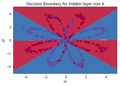
png
1 | # Print accuracy |
Accuracy: 90%调参:隐藏层神经元个数
1 | # This may take about 2 minutes to run |
Accuracy for 1 hidden units: 67.5 %
Accuracy for 2 hidden units: 67.25 %
Accuracy for 3 hidden units: 90.75 %
Accuracy for 4 hidden units: 90.5 %
Accuracy for 5 hidden units: 91.25 %
Accuracy for 20 hidden units: 90.0 %
Accuracy for 50 hidden units: 90.75 %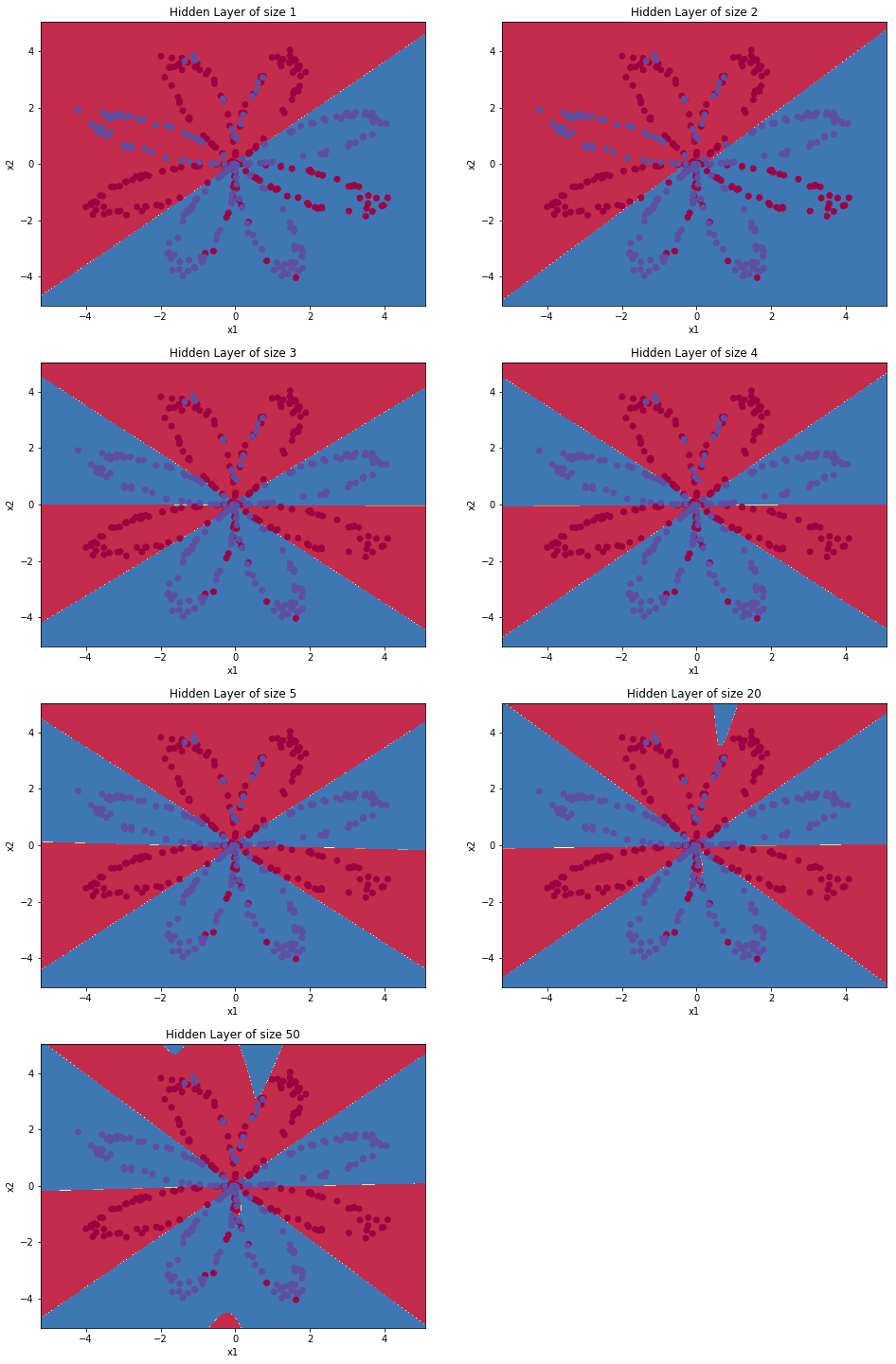
png
测试其他数据集
1 | # Datasets |
png
结论
- 隐藏层神经元个数越多,越容易拟合训练数据,知道过拟合
- 最佳的隐藏层神经元个数大概为5,既可以很好的拟合数据,也不会引入过拟合
- 另一种既可以使用大的神经网络,又可以避免过拟合的方法是正则化。
附录
非线性激活函数的种类
sigmoid函数
\[ g(z) = \frac{1}{1+e^{-z}} \] 导数为: \[ g'(z) = g(z)(1-g(z)) \]tanh函数
\[ g(z) = tanh(z) = \frac{e^z-e^{-z}}{e^z+e^{-z}} = 2*sigmoid(z) - 1 \] 导数为: \[ g'(z) = 1-g^2(z) \]ReLU函数 \[ g(z) = max(0,z) \] 导数为: \[ g'(z) = \begin{cases} 0 & \text{if}\ z < 0 \\ 1 & \text{if}\ z > 0 \\ \text{not defined} & \text{otherwise} \\ \end{cases} \]
Leaky ReLU(Rectified Linear Unit)函数 \[ g(z) = max(\alpha z,z)\ 0\le z \le 1 \] 导数为: \[ g'(z) = \begin{cases} \alpha & \text{if}\ z < 0 \\ 1 & \text{if}\ z > 0 \\ \text{not defined} & \text{otherwise} \\ \end{cases} \]
- 大部分情况下,tanh函数(输出均值为0)都优于sigmoid函数,除非在输出层进行二分类时,必须使用sigmoid函数
- 当z很大或者很小时,sigmoid和tanh函数的梯度都很小,导致收敛速度很慢,因此默认情况下都是使用ReLU函数
1 | z = np.arange(-20,20,0.1) |
[<matplotlib.lines.Line2D at 0x7f065e7bdf60>]
png

png

png

png
为何要在隐藏层使用非线性激活函数
正传过程中,对一个样本 \(x^{(i)}\): \[z^{[1] (i)} = W^{[1]} x^{(i)} + b^{[1] (i)}\tag{1}\] \[a^{[1] (i)} = g^{[1]}(z^{[1] (i)})\tag{2}\] \[z^{[2] (i)} = W^{[2]} a^{[1] (i)} + b^{[2] (i)}\tag{3}\] \[\hat{y}^{(i)} = a^{[2] (i)} = g^{[2]}(z^{ [2] (i)})\tag{4}\] 当\(g^{[1]}=g^{[2]}=I\),可以证明: \[ a^{[2] (i)} = W'x^{(i)}+b' = (W^{[1]}W^{[2]})x^{(i)}+(W^{[2]}b^{[1] (i)}+b^{[2] (i)}) \] 也是说,当采用线性激活函数,神经网络等效于线性回归。 当输出为sigmoid函数,但是隐藏层使用线性激活函数,则深度神经网络依然和逻辑回归等效。
为何不能将深度神经网络的模型参数初始化为0
在逻辑回归算法中,模型参数初始化为0,但是在多于一层的神经网络中,不能将模型参数初始化为0。原因是:当W初始化为0,各个神经元计算的结果相同,W的更新量每一行也相同,也就没有必要增加神经元的个数了,这是著名的Symmetric breaking问题。解决办法是初始化W为随机向量,例如\(W^{[1]}=np.random.randn(n^{[1]},n^{[0]})*0.01;b^{[1]}=np.zeros((n^{[1]},1))\),其中取比较小的\(0.01\)是为了使得作为sigmoid函数的输入不要太大,不然容易导致梯度饱和(梯度接近于0),降低收敛速度。
参考资料
- 吴恩达,coursera深度学习课程