搭建深度神经网络

深度神经网络是指多于一个隐藏层的神经网络。本文将详细介绍深度神经网络的基本原理及实现。涉及到模型的初始化、梯度的计算、激活函数的求导等内容。

符号 - 上标 \([l]\) 代表第 \(l\) 层的数值. - 例如: \(a^{[L]}\) 表示第 \(L\) 层激活函数的输出. \(W^{[L]}\)\(b^{[L]}\) 表示第 \(L\) 层的参数. - 上标 \((i)\) 表示第 \(i\) 样本. - 例如: \(x^{(i)}\) 表示第 \(i\) 训练样本. - 下标 \(i\) 表示向量的第 \(i\) 个元素. - 例如: \(a^{[l]}_i\) 表示第\(l\)层第\(i\)个神经元的输出.

1
2
3
4
5
6
7
8
9
10
11
12
13
14
15
import numpy as np
import h5py
import matplotlib.pyplot as plt
from testCases_v2 import *
from dnn_utils_v2 import sigmoid, sigmoid_backward, relu, relu_backward

%matplotlib inline
plt.rcParams['figure.figsize'] = (5.0, 4.0) # set default size of plots
plt.rcParams['image.interpolation'] = 'nearest'
plt.rcParams['image.cmap'] = 'gray'

%load_ext autoreload
%autoreload 2

np.random.seed(1)

网络结构

为建立神经网络,需要实现几个子函数,它们具体的功能包括:

  • 初始化模型参数.
  • 实现正传模块(下图紫色部分)Implement the forward propagation module (shown in purple in the figure below).
    • 实现正传中的线性部分(得到 \(Z^{[l]}\)).
    • 实现激活函数(relu/sigmoid).
    • 结合前面两步形成一个新的正传函数[LINEAR->ACTIVATION].
    • 将 [LINEAR->RELU] 正传函数重复 L-1 次 (从第 1 层到 L-1层) 并在最后一层添加 [LINEAR->SIGMOID] (第 \(L\)层). 那样就形成了 L_model_forward 函数.
  • 计算损失函数.
  • 实现反传模块 (下图红色部分).
    • 计算反传中的线性部分.
    • 实现激活函数的梯度(relu_backward/sigmoid_backward)
    • 结合签名两步实现一个新的反传函数 [LINEAR->ACTIVATION].
    • 将 [LINEAR->RELU] 反传 L-1 次并在最后一层加入[LINEAR->SIGMOID] 反传过程,那样形成了一个新的L_model_backward 函数
  • 更新模型.
Figure 1


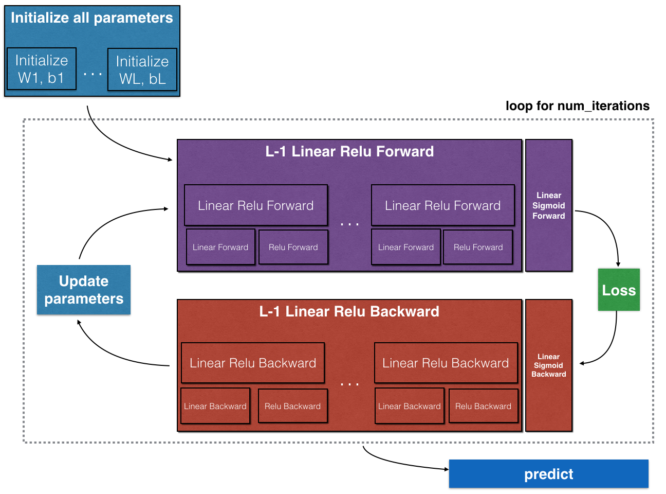
注意 在一个正传函数中,都有对应的反传函数,因此每一步都需要寄存一些值,用于计算梯度。

初始化

分别介绍两层和多层网络的参数初始化

两层网络

1
2
3
4
5
6
7
8
9
10
11
12
13
14
15
16
17
18
19
20
21
22
23
24
25
26
27
28
29
30
31
32
33
34
35
36
37
# GRADED FUNCTION: initialize_parameters

def initialize_parameters(n_x, n_h, n_y):
"""
Argument:
n_x -- size of the input layer
n_h -- size of the hidden layer
n_y -- size of the output layer

Returns:
parameters -- python dictionary containing your parameters:
W1 -- weight matrix of shape (n_h, n_x)
b1 -- bias vector of shape (n_h, 1)
W2 -- weight matrix of shape (n_y, n_h)
b2 -- bias vector of shape (n_y, 1)
"""

np.random.seed(1)

### START CODE HERE ### (≈ 4 lines of code)
W1 = np.random.randn(n_h, n_x) * 0.01
b1 = np.zeros((n_h, 1))
W2 = np.random.randn(n_y, n_h) * 0.01
b2 = np.zeros((n_y, 1))
### END CODE HERE ###

assert(W1.shape == (n_h, n_x))
assert(b1.shape == (n_h, 1))
assert(W2.shape == (n_y, n_h))
assert(b2.shape == (n_y, 1))

parameters = {"W1": W1,
"b1": b1,
"W2": W2,
"b2": b2}

return parameters
1
2
3
4
5
parameters = initialize_parameters(2,2,1)
print("W1 = " + str(parameters["W1"]))
print("b1 = " + str(parameters["b1"]))
print("W2 = " + str(parameters["W2"]))
print("b2 = " + str(parameters["b2"]))
W1 = [[ 0.01624345 -0.00611756]
 [-0.00528172 -0.01072969]]
b1 = [[ 0.]
 [ 0.]]
W2 = [[ 0.00865408 -0.02301539]]
b2 = [[ 0.]]

\(L\)层网络

假定 \(n^{[l]}\) 是第 \(l\)层的神经元个数. 当输入 \(X\) 大小为 \((12288, 209)\) (其中 \(m=209\) 为样本数) ,则:

<tr>
    <td>  </td> 
    <td> **Shape of W** </td> 
    <td> **Shape of b**  </td> 
    <td> **Activation** </td>
    <td> **Shape of Activation** </td> 
<tr>

<tr>
    <td> **Layer 1** </td> 
    <td> $(n^{[1]},12288)$ </td> 
    <td> $(n^{[1]},1)$ </td> 
    <td> $Z^{[1]} = W^{[1]}  X + b^{[1]} $ </td> 
    
    <td> $(n^{[1]},209)$ </td> 
<tr>

<tr>
    <td> **Layer 2** </td> 
    <td> $(n^{[2]}, n^{[1]})$  </td> 
    <td> $(n^{[2]},1)$ </td> 
    <td>$Z^{[2]} = W^{[2]} A^{[1]} + b^{[2]}$ </td> 
    <td> $(n^{[2]}, 209)$ </td> 
<tr>

   <tr>
    <td> $\vdots$ </td> 
    <td> $\vdots$  </td> 
    <td> $\vdots$  </td> 
    <td> $\vdots$</td> 
    <td> $\vdots$  </td> 
<tr>
    <td> **Layer L-1** </td> 
    <td> $(n^{[L-1]}, n^{[L-2]})$ </td> 
    <td> $(n^{[L-1]}, 1)$  </td> 
    <td>$Z^{[L-1]} =  W^{[L-1]} A^{[L-2]} + b^{[L-1]}$ </td> 
    <td> $(n^{[L-1]}, 209)$ </td> 
<tr>
    <td> **Layer L** </td> 
    <td> $(n^{[L]}, n^{[L-1]})$ </td> 
    <td> $(n^{[L]}, 1)$ </td>
    <td> $Z^{[L]} =  W^{[L]} A^{[L-1]} + b^{[L]}$</td>
    <td> $(n^{[L]}, 209)$  </td> 
<tr>

Python在计算 \(W X + b\)时, 使用了广播功能. 例如:

\[ W = \begin{bmatrix} j & k & l\\ m & n & o \\ p & q & r \end{bmatrix}\;\;\; X = \begin{bmatrix} a & b & c\\ d & e & f \\ g & h & i \end{bmatrix} \;\;\; b =\begin{bmatrix} s \\ t \\ u \end{bmatrix}\tag{2}\]

那么 \(WX + b\) 将为:

\[ WX + b = \begin{bmatrix} (ja + kd + lg) + s & (jb + ke + lh) + s & (jc + kf + li)+ s\\ (ma + nd + og) + t & (mb + ne + oh) + t & (mc + nf + oi) + t\\ (pa + qd + rg) + u & (pb + qe + rh) + u & (pc + qf + ri)+ u \end{bmatrix}\tag{3} \]

1
2
3
4
5
6
7
8
9
10
11
12
13
14
15
16
17
18
19
20
21
22
23
24
25
26
27
28
# GRADED FUNCTION: initialize_parameters_deep

def initialize_parameters_deep(layer_dims):
"""
Arguments:
layer_dims -- python array (list) containing the dimensions of each layer in our network

Returns:
parameters -- python dictionary containing your parameters "W1", "b1", ..., "WL", "bL":
Wl -- weight matrix of shape (layer_dims[l], layer_dims[l-1])
bl -- bias vector of shape (layer_dims[l], 1)
"""

np.random.seed(3)
parameters = {}
L = len(layer_dims) # number of layers in the network

for l in range(1, L):
### START CODE HERE ### (≈ 2 lines of code)
parameters['W' + str(l)] = np.random.randn(layer_dims[l], layer_dims[l-1]) * 0.01
parameters['b' + str(l)] = np.zeros((layer_dims[l], 1))
### END CODE HERE ###

assert(parameters['W' + str(l)].shape == (layer_dims[l], layer_dims[l-1]))
assert(parameters['b' + str(l)].shape == (layer_dims[l], 1))


return parameters
1
2
3
4
5
parameters = initialize_parameters_deep([5,4,3])
print("W1 = " + str(parameters["W1"]))
print("b1 = " + str(parameters["b1"]))
print("W2 = " + str(parameters["W2"]))
print("b2 = " + str(parameters["b2"]))
W1 = [[ 0.01788628  0.0043651   0.00096497 -0.01863493 -0.00277388]
 [-0.00354759 -0.00082741 -0.00627001 -0.00043818 -0.00477218]
 [-0.01313865  0.00884622  0.00881318  0.01709573  0.00050034]
 [-0.00404677 -0.0054536  -0.01546477  0.00982367 -0.01101068]]
b1 = [[ 0.]
 [ 0.]
 [ 0.]
 [ 0.]]
W2 = [[-0.01185047 -0.0020565   0.01486148  0.00236716]
 [-0.01023785 -0.00712993  0.00625245 -0.00160513]
 [-0.00768836 -0.00230031  0.00745056  0.01976111]]
b2 = [[ 0.]
 [ 0.]
 [ 0.]]

正传模块

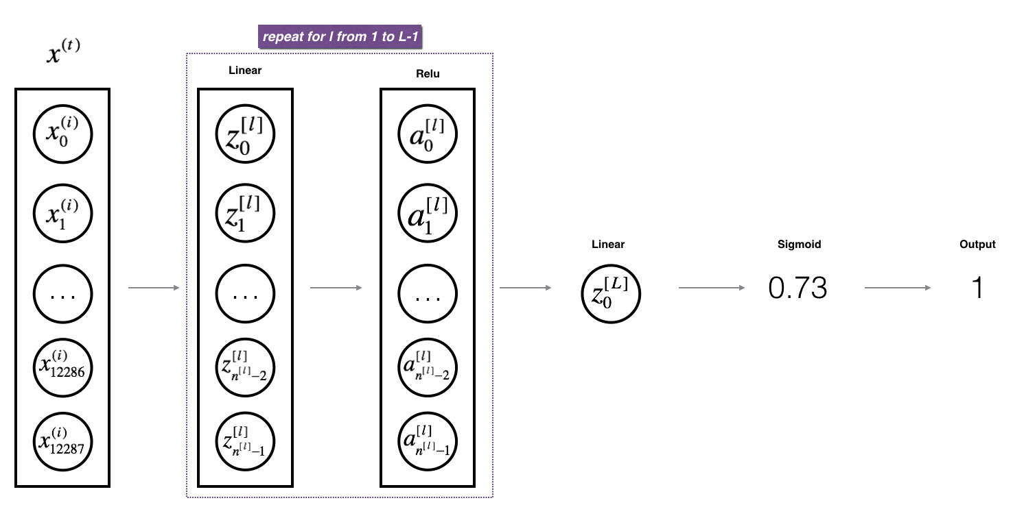
对所有样本向量化之后的正传模块实现如下公式:

\[Z^{[l]} = W^{[l]}A^{[l-1]} +b^{[l]}\tag{4}\]

其中 \(A^{[0]} = X\).

线性正传

1
2
3
4
5
6
7
8
9
10
11
12
13
14
15
16
17
18
19
20
21
22
23
24
# GRADED FUNCTION: linear_forward

def linear_forward(A, W, b):
"""
Implement the linear part of a layer's forward propagation.

Arguments:
A -- activations from previous layer (or input data): (size of previous layer, number of examples)
W -- weights matrix: numpy array of shape (size of current layer, size of previous layer)
b -- bias vector, numpy array of shape (size of the current layer, 1)

Returns:
Z -- the input of the activation function, also called pre-activation parameter
cache -- a python dictionary containing "A", "W" and "b" ; stored for computing the backward pass efficiently
"""

### START CODE HERE ### (≈ 1 line of code)
Z = np.dot(W, A) + b
### END CODE HERE ###

assert(Z.shape == (W.shape[0], A.shape[1]))
cache = (A, W, b)

return Z, cache
1
2
3
4
A, W, b = linear_forward_test_case()

Z, linear_cache = linear_forward(A, W, b)
print("Z = " + str(Z))
Z = [[ 3.26295337 -1.23429987]]

线性正传+激活函数

实现正传 LINEAR->ACTIVATION .数学关系是: \(A^{[l]} = g(Z^{[l]}) = g(W^{[l]}A^{[l-1]} +b^{[l]})\) 其中激活函数 "g" 可以是 sigmoid() 或者 relu()

1
2
3
4
5
6
7
8
9
10
11
12
13
14
15
16
17
18
19
20
21
22
23
24
25
26
27
28
29
30
31
32
33
34
35
36
# GRADED FUNCTION: linear_activation_forward

def linear_activation_forward(A_prev, W, b, activation):
"""
Implement the forward propagation for the LINEAR->ACTIVATION layer

Arguments:
A_prev -- activations from previous layer (or input data): (size of previous layer, number of examples)
W -- weights matrix: numpy array of shape (size of current layer, size of previous layer)
b -- bias vector, numpy array of shape (size of the current layer, 1)
activation -- the activation to be used in this layer, stored as a text string: "sigmoid" or "relu"

Returns:
A -- the output of the activation function, also called the post-activation value
cache -- a python dictionary containing "linear_cache" and "activation_cache";
stored for computing the backward pass efficiently
"""

if activation == "sigmoid":
# Inputs: "A_prev, W, b". Outputs: "A, activation_cache".
### START CODE HERE ### (≈ 2 lines of code)
Z, linear_cache = linear_forward(A_prev, W, b)
A, activation_cache = sigmoid(Z)
### END CODE HERE ###

elif activation == "relu":
# Inputs: "A_prev, W, b". Outputs: "A, activation_cache".
### START CODE HERE ### (≈ 2 lines of code)
Z, linear_cache = linear_forward(A_prev, W, b)
A, activation_cache = relu(Z)
### END CODE HERE ###

assert (A.shape == (W.shape[0], A_prev.shape[1]))
cache = (linear_cache, activation_cache)

return A, cache
1
2
3
4
5
6
7
A_prev, W, b = linear_activation_forward_test_case()

A, linear_activation_cache = linear_activation_forward(A_prev, W, b, activation = "sigmoid")
print("With sigmoid: A = " + str(A))

A, linear_activation_cache = linear_activation_forward(A_prev, W, b, activation = "relu")
print("With ReLU: A = " + str(A))
With sigmoid: A = [[ 0.96890023  0.11013289]]
With ReLU: A = [[ 3.43896131  0.        ]]

\(L\)层模型

为了实现 \(L\)层神经网络,可以复制前面的正传+ReLU激活函数 (linear_activation_forward + RELU) \(L-1\) 次, 然后接上 linear_activation_forward + SIGMOID.

Figure 2 : [LINEAR -> RELU] \(\times\) (L-1) -> LINEAR -> SIGMOID model


1
2
3
4
5
6
7
8
9
10
11
12
13
14
15
16
17
18
19
20
21
22
23
24
25
26
27
28
29
30
31
32
33
34
35
36
37
38
39
40
41
42
43
44
45
46
# GRADED FUNCTION: L_model_forward

def L_model_forward(X, parameters):
"""
Implement forward propagation for the [LINEAR->RELU]*(L-1)->LINEAR->SIGMOID computation

Arguments:
X -- data, numpy array of shape (input size, number of examples)
parameters -- output of initialize_parameters_deep()

Returns:
AL -- last post-activation value
caches -- list of caches containing:
every cache of linear_relu_forward() (there are L-1 of them, indexed from 0 to L-2)
the cache of linear_sigmoid_forward() (there is one, indexed L-1)
"""

caches = []
A = X
L = len(parameters) // 2 # number of layers in the neural network

# Implement [LINEAR -> RELU]*(L-1). Add "cache" to the "caches" list.
for l in range(1, L):
A_prev = A
### START CODE HERE ### (≈ 2 lines of code)
A, cache = linear_activation_forward(A_prev,
parameters["W" + str(l)],
parameters["b" + str(l)],
activation='relu')
caches.append(cache)

### END CODE HERE ###

# Implement LINEAR -> SIGMOID. Add "cache" to the "caches" list.
### START CODE HERE ### (≈ 2 lines of code)
AL, cache = linear_activation_forward(A,
parameters["W" + str(L)],
parameters["b" + str(L)],
activation='sigmoid')
caches.append(cache)

### END CODE HERE ###

assert(AL.shape == (1,X.shape[1]))

return AL, caches
1
2
3
4
X, parameters = L_model_forward_test_case()
AL, caches = L_model_forward(X, parameters)
print("AL = " + str(AL))
print("Length of caches list = " + str(len(caches)))
AL = [[ 0.17007265  0.2524272 ]]
Length of caches list = 2

代价函数

交叉熵代价函数 \(J\): \[-\frac{1}{m} \sum\limits_{i = 1}^{m} (y^{(i)}\log\left(a^{[L] (i)}\right) + (1-y^{(i)})\log\left(1- a^{[L](i)}\right)) \tag{7}\]

1
2
3
4
5
6
7
8
9
10
11
12
13
14
15
16
17
18
19
20
21
22
23
24
25
# GRADED FUNCTION: compute_cost

def compute_cost(AL, Y):
"""
Implement the cost function defined by equation (7).

Arguments:
AL -- probability vector corresponding to your label predictions, shape (1, number of examples)
Y -- true "label" vector (for example: containing 0 if non-cat, 1 if cat), shape (1, number of examples)

Returns:
cost -- cross-entropy cost
"""

m = Y.shape[1]

# Compute loss from aL and y.
### START CODE HERE ### (≈ 1 lines of code)
cost = (-1./ m) * np.sum(np.multiply(Y, np.log(AL)) + np.multiply((1-Y), np.log( 1-AL)))
### END CODE HERE ###

cost = np.squeeze(cost) # To make sure your cost's shape is what we expect (e.g. this turns [[17]] into 17).
assert(cost.shape == ())

return cost
1
2
3
Y, AL = compute_cost_test_case()

print("cost = " + str(compute_cost(AL, Y)))
cost = 0.414931599615

反传模块

反传模块的作用是计算损失函数关于参数的梯度

提醒:
Figure 3 : LINEAR->RELU->LINEAR->SIGMOID 正传和反传过程:
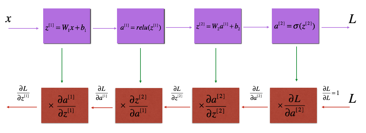
紫色方块表示正传过程, 红色模块表示反传过程.