本文介绍深度神经网络的一个主要应用:计算机视觉。对比逻辑回归,浅层神经网络在图像分类中的性能,说明深度神经网络在图像分类中的应用价值。
预处理
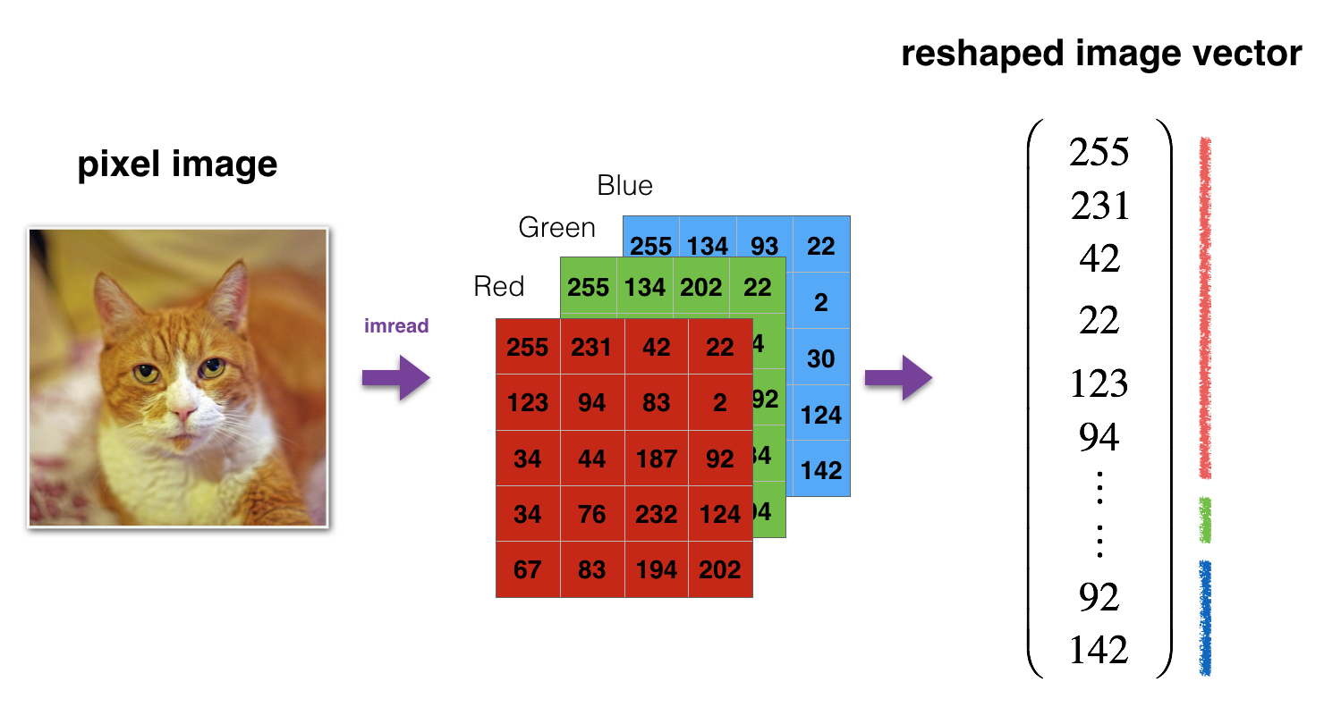
预处理包括:将图像向量化以及对像素的标准化
1 | import time |
1 | train_x_orig, train_y, test_x_orig, test_y, classes = load_data() |
1 | # Example of a picture |
y = 0. It's a non-cat picture.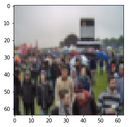
png
1 | # Explore your dataset |
Number of training examples: 209
Number of testing examples: 50
Each image is of size: (64, 64, 3)
train_x_orig shape: (209, 64, 64, 3)
train_y shape: (1, 209)
test_x_orig shape: (50, 64, 64, 3)
test_y shape: (1, 50)
1 | # Reshape the training and test examples |
train_x's shape: (12288, 209)
test_x's shape: (12288, 50)
神经网络的架构
本文对比两种架构,一种是2层神经网络,一种是更深的神经网络。
两层神经网络
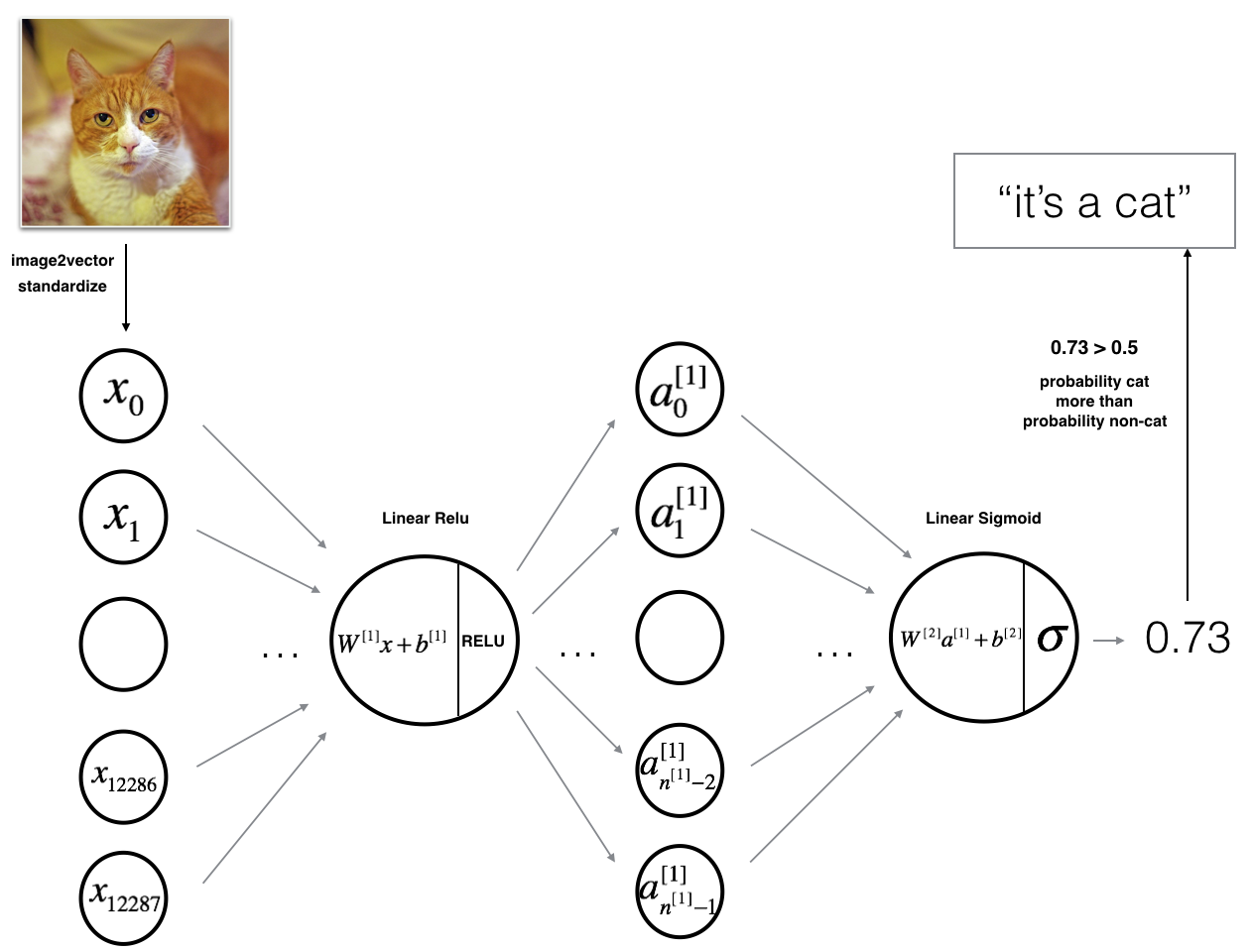
模型可以总结为: INPUT -> LINEAR -> RELU -> LINEAR -> SIGMOID -> OUTPUT.
图2的细节: - 输入图像 (64,64,3) 整形为大小为 \((12288,1)\) 的向量. - 对应的向量: \([x_0,x_1,...,x_{12287}]^T\) 乘以大小为\((n^{[1]}, 12288)\)的加权矩阵 \(W^{[1]}\). - 加上偏移量,并取RELU: \([a_0^{[1]}, a_1^{[1]},..., a_{n^{[1]}-1}^{[1]}]^T\). - 重复上述过程. - 乘以\(W^{[2]}\) 并加上截距 (偏移量). - 最终取结果的sigmoid响应. 如果大于 0.5, 分类为猫.
\(L\)层深度神经网络
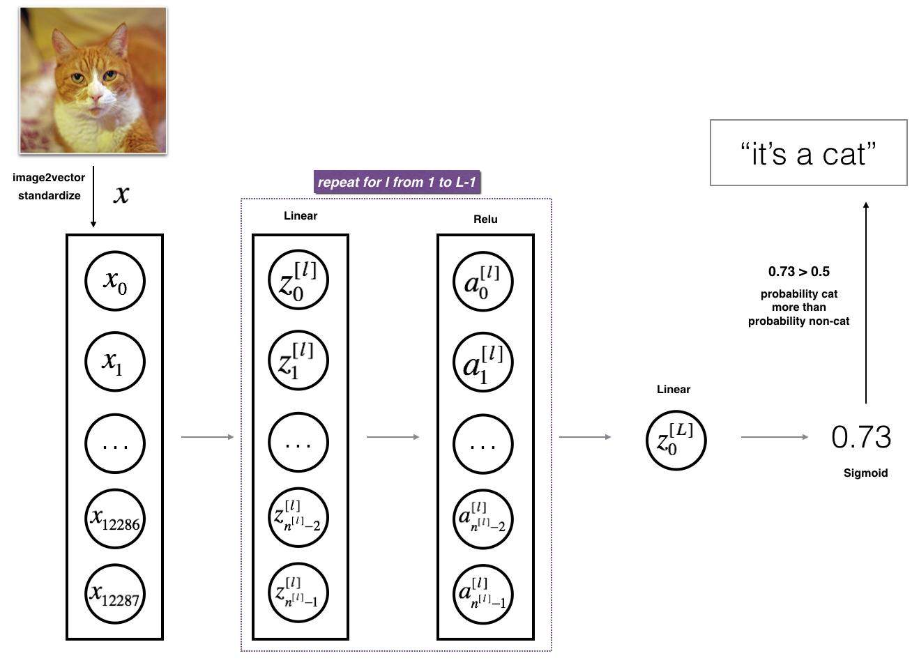
模型可以总结为: [LINEAR -> RELU] \(\times\) (L-1) -> LINEAR -> SIGMOID
图3的细节: - 输入图像 (64,64,3) 整形为大小为 \((12288,1)\) 的向量. - 对应的向量: \([x_0,x_1,...,x_{12287}]^T\) 乘以大小为\((n^{[1]}, 12288)\)的加权矩阵 \(W^{[1]}\). - 加上偏移量,并取RELU: \([a_0^{[1]}, a_1^{[1]},..., a_{n^{[1]}-1}^{[1]}]^T\). - 根据模型的架构,对每对 \((W^{[l]}, b^{[l]})\) 重复多次. - 最终, 取最后一层线性单元的sigmoid响应. 如果大于 0.5, 分类为猫.
实现方法
方法如下: 1. 初始化参数、定义超参 2. 循环num_iterations次: a. 正传 b. 计算代价函数 c. 反传 d. 更新模型 4. 利用训练的参数进行预测
两层网络
1 | ### CONSTANTS DEFINING THE MODEL #### |
1 | # GRADED FUNCTION: two_layer_model |
1 | parameters = two_layer_model(train_x, train_y, layers_dims = (n_x, n_h, n_y), num_iterations = 2500, print_cost=True) |
Cost after iteration 0: 0.6930497356599888
Cost after iteration 100: 0.6464320953428849
Cost after iteration 200: 0.6325140647912678
Cost after iteration 300: 0.6015024920354665
Cost after iteration 400: 0.5601966311605748
Cost after iteration 500: 0.5158304772764729
Cost after iteration 600: 0.4754901313943325
Cost after iteration 700: 0.43391631512257495
Cost after iteration 800: 0.4007977536203889
Cost after iteration 900: 0.3580705011323798
Cost after iteration 1000: 0.33942815383664127
Cost after iteration 1100: 0.3052753636196264
Cost after iteration 1200: 0.27491377282130164
Cost after iteration 1300: 0.24681768210614818
Cost after iteration 1400: 0.19850735037466105
Cost after iteration 1500: 0.17448318112556663
Cost after iteration 1600: 0.17080762978096006
Cost after iteration 1700: 0.11306524562164738
Cost after iteration 1800: 0.09629426845937156
Cost after iteration 1900: 0.08342617959726865
Cost after iteration 2000: 0.07439078704319083
Cost after iteration 2100: 0.06630748132267933
Cost after iteration 2200: 0.05919329501038172
Cost after iteration 2300: 0.05336140348560558
Cost after iteration 2400: 0.04855478562877019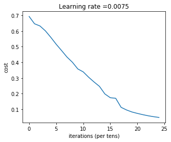
png
1 | predictions_train = predict(train_x, train_y, parameters) |
Accuracy: 1.01 | predictions_test = predict(test_x, test_y, parameters) |
Accuracy: 0.72注意: 在1500步的结果也许可以得到更好的准确度,提前终止也是一种避免过拟合的方法。两层神经网络的表现优于逻辑回归(前面的结果70%)。
L层深层网络
1 | ### CONSTANTS ### |
1 | # GRADED FUNCTION: L_layer_model |
1 | parameters = L_layer_model(train_x, train_y, layers_dims, num_iterations = 2500, print_cost = True) |
Cost after iteration 0: 0.771749
Cost after iteration 100: 0.672053
Cost after iteration 200: 0.648263
Cost after iteration 300: 0.611507
Cost after iteration 400: 0.567047
Cost after iteration 500: 0.540138
Cost after iteration 600: 0.527930
Cost after iteration 700: 0.465477
Cost after iteration 800: 0.369126
Cost after iteration 900: 0.391747
Cost after iteration 1000: 0.315187
Cost after iteration 1100: 0.272700
Cost after iteration 1200: 0.237419
Cost after iteration 1300: 0.199601
Cost after iteration 1400: 0.189263
Cost after iteration 1500: 0.161189
Cost after iteration 1600: 0.148214
Cost after iteration 1700: 0.137775
Cost after iteration 1800: 0.129740
Cost after iteration 1900: 0.121225
Cost after iteration 2000: 0.113821
Cost after iteration 2100: 0.107839
Cost after iteration 2200: 0.102855
Cost after iteration 2300: 0.100897
Cost after iteration 2400: 0.092878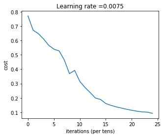
png
1 | pred_train = predict(train_x, train_y, parameters) |
Accuracy: 0.9856459330141 | pred_test = predict(test_x, test_y, parameters) |
Accuracy: 0.8注意: 可以看出,结果要优于两层网络。进一步的,可以通过调参(学习率、层数、神经元个数、迭代次数等)改善结果。
结果分析
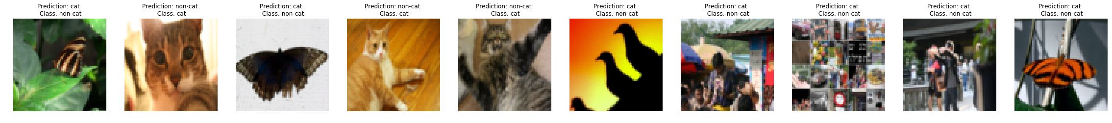
1 | print_mislabeled_images(classes, test_x, test_y, pred_test) |
png
分析结果发现,错分的图像包括:
- 猫的姿势特殊
- 猫出现在和它类似的背景上
- 猫的颜色和品种特殊
- 摄像头角度问题
- 图像的色度
- 尺度问题
通过分析,可以进一步采集新数据或者合成数据,改善性能。
测试用户的图像
1 | ## START CODE HERE ## |
Accuracy: 1.0
y = 1.0, your L-layer model predicts a "cat" picture.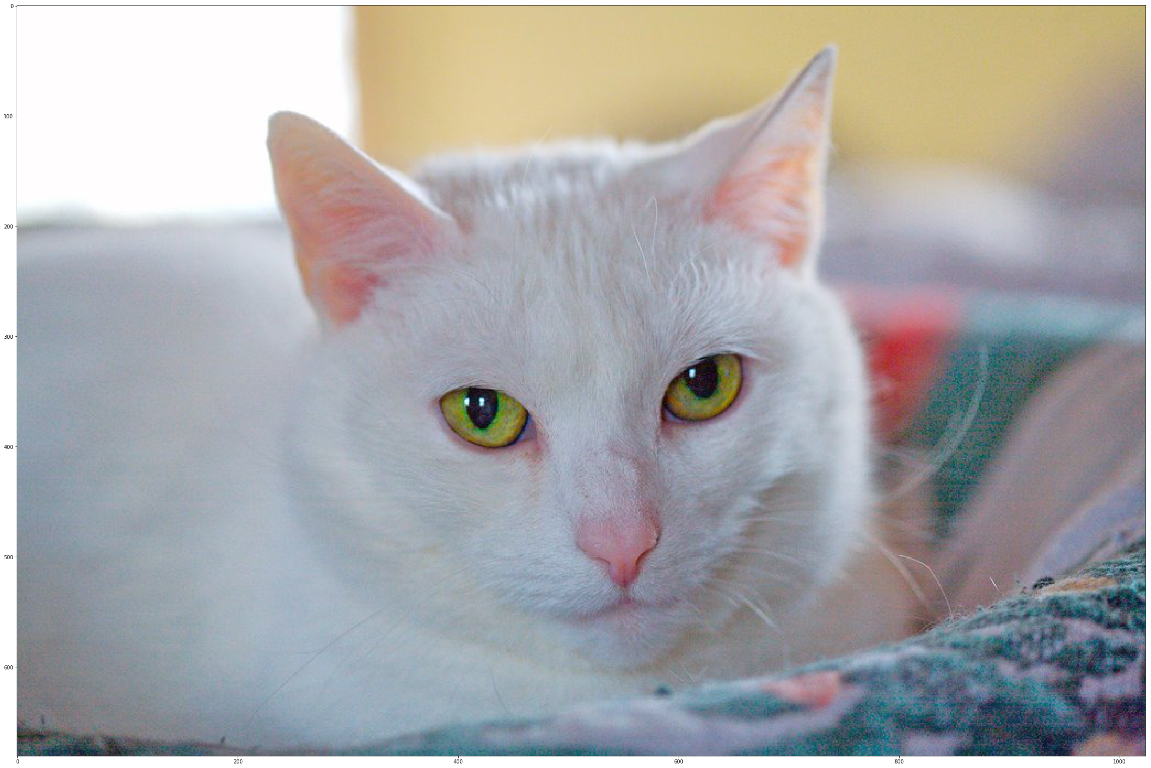
png
参考资料
- 吴恩达,coursera深度学习课程