本文介绍一个提高深度神经网络性能的因素——正则化。深度神经网络十分灵活,增加网络深度可以很好地拟合训练数据,但是过拟合是一个很严重的问题,也就是说泛化能力不足。本文介绍两种解决方案:一种是用L2范数对模型参数进行正则化;另一种是用Dropout策略在每次迭代过程中随机丢失一部分神经元。两种方案都可以达到解决过拟合问题的目的。
数据加载
1 | # import packages |
/media/seisinv/Data/svn/ai/learn/dl_ng/reg_utils.py:85: SyntaxWarning: assertion is always true, perhaps remove parentheses?
  assert(parameters['W' + str(l)].shape == layer_dims[l], layer_dims[l-1])
/media/seisinv/Data/svn/ai/learn/dl_ng/reg_utils.py:86: SyntaxWarning: assertion is always true, perhaps remove parentheses?
  assert(parameters['W' + str(l)].shape == layer_dims[l], 1)
1 | train_X, train_Y, test_X, test_Y = load_2D_dataset() |
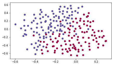
png
不带正则化的模型
1 | def model(X, Y, learning_rate = 0.3, num_iterations = 30000, print_cost = True, lambd = 0, keep_prob = 1): |
1 | parameters = model(train_X, train_Y) |
Cost after iteration 0: 0.6557412523481002
Cost after iteration 10000: 0.16329987525724216
Cost after iteration 20000: 0.13851642423255986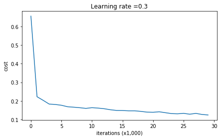
png
On the training set:
Accuracy: 0.947867298578
On the test set:
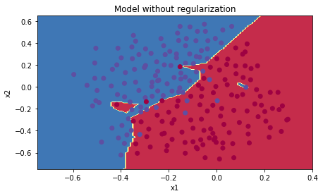
Accuracy: 0.9151 | plt.title("Model without regularization") |
png
小结:不带正则化的模型对训练数据过拟合,不仅拟合了正常的数据点,也拟合了噪音。
L2正则化
避免过拟合的常规做法是做L2正则化。代价函数从: \[J = -\frac{1}{m} \sum\limits_{i = 1}^{m} \large{(}\small y^{(i)}\log\left(a^{[L](i)}\right) + (1-y^{(i)})\log\left(1- a^{[L](i)}\right) \large{)} \tag{1}\] 变为: \[J_{regularized} = \small \underbrace{-\frac{1}{m} \sum\limits_{i = 1}^{m} \large{(}\small y^{(i)}\log\left(a^{[L](i)}\right) + (1-y^{(i)})\log\left(1- a^{[L](i)}\right) \large{)} }_\text{cross-entropy cost} + \underbrace{\frac{1}{m} \frac{\lambda}{2} \sum\limits_l\sum\limits_k\sum\limits_j W_{k,j}^{[l]2} }_\text{L2 regularization cost} \tag{2}\]
梯度增加一项: \[\frac{d}{dW} ( \frac{1}{2}\frac{\lambda}{m} W^2) = \frac{\lambda}{m} W\]
对应的算法也称为"weight decay"梯度下降法
1 | # GRADED FUNCTION: compute_cost_with_regularization |
1 | A3, Y_assess, parameters = compute_cost_with_regularization_test_case() |
cost = 1.786485945161 | # GRADED FUNCTION: backward_propagation_with_regularization |
1 | X_assess, Y_assess, cache = backward_propagation_with_regularization_test_case() |
dW1 = [[-0.25604646  0.12298827 -0.28297129]
 [-0.17706303  0.34536094 -0.4410571 ]]
dW2 = [[ 0.79276486  0.85133918]
 [-0.0957219  -0.01720463]
 [-0.13100772 -0.03750433]]
dW3 = [[-1.77691347 -0.11832879 -0.09397446]]
1 | parameters = model(train_X, train_Y, lambd = 0.7) |
Cost after iteration 0: 0.6974484493131264
Cost after iteration 10000: 0.2684918873282239
Cost after iteration 20000: 0.26809163371273015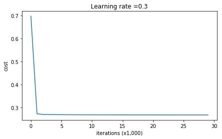
png
On the train set:
Accuracy: 0.938388625592
On the test set:
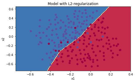
Accuracy: 0.931 | plt.title("Model with L2-regularization") |
png
小结:
- 模型不再过拟合数据,泛化精度得到提升
- \(\lambda\)是一个超参,需要使用dev数据集进行调整
- L2正则化使得决策边界更加平滑。当\(\lambda\)太大,也有可能使得决策边界过平滑,导致模型偏差太大
- L2正则化基于假设:小权值的模型比大权值模型更简单。因此通过在代价函数中压制权值的平方和,达到驱使权值变小的目的,最终产生一个平滑的模型(也即:当输入发生变化时,输出变化更加缓慢。
Dropout
Dropout是深度学习中特有的一种正则化手段。该方法在每次迭代过程中随机关闭一些神经元。
在每次迭代过程中, 以\(1 - keep\_prob\)的概率关闭 (也即令它为0) 一层中这个神经元或者以\(keep\_prob\)的概率保留这个神经元(这里为50%). 丢失的神经元在这次迭代中既不会对正传、也不会对反传产生影响.
第\(1\)层: 关闭40%的神经元. 第3层: 关闭20%的神经元.
Drop-out的基本思想是:只有一部分神经元训练模型,使得输出不过度依赖于任何特征,也就使得权值分布均匀,起到压缩权值的作用,类似于L2正则化。
带dropout的正传播过程
本文采用3层神经网络,并对第1和第2个隐藏层实施dropout操作。具体分为以下4步:
- 利用函数
np.random.rand()生成矩阵 \(D^{[1]}\) ,其维度和\(A^{[1]}\)相同.
- 通过阈值,使矩阵\(D^{[1]}\) 中的元素
1-keep_prob的概率为0,keep_prob的概率为1.
- 令 \(A^{[1]}\) 为 \(A^{[1]} * D^{[1]}\).
- 将 \(A^{[1]}\) 除以
keep_prob. 这样做的目的是为了保证drop-out之后的输出和没有drop-out的输出具有相同的期望。该方法也成为inverted dropout
1 | # GRADED FUNCTION: forward_propagation_with_dropout |
1 | X_assess, parameters = forward_propagation_with_dropout_test_case() |
A3 = [[ 0.36974721 0.00305176 0.04565099 0.49683389 0.36974721]]带dropout的反传播过程
使用寄存中的\(D^{[1]}\) and \(D^{[2]}\) 矩阵,应用以下2步实施反传播:
- 之前在正传过程中对
A1应用 \(D^{[1]}\). 因此反传过程中也需要对dA1应用\(D^{[1]}\)关闭相同的神经元。
- 之前在正传过程中将
A1除以keep_prob,因此在反传过程中,也需要再次对dA1除以keep_prob(数值解释是:如果 \(A^{[1]}\) 除以keep_prob, 那么他的导数\(dA^{[1]}\)也应该除以keep_prob).
1 | # GRADED FUNCTION: backward_propagation_with_dropout |
1 | X_assess, Y_assess, cache = backward_propagation_with_dropout_test_case() |
dA1 = [[ 0.36544439  0.         -0.00188233  0.         -0.17408748]
 [ 0.65515713  0.         -0.00337459  0.         -0.        ]]
dA2 = [[ 0.58180856  0.         -0.00299679  0.         -0.27715731]
 [ 0.          0.53159854 -0.          0.53159854 -0.34089673]
 [ 0.          0.         -0.00292733  0.         -0.        ]]
1 | parameters = model(train_X, train_Y, keep_prob = 0.86, learning_rate = 0.3) |
Cost after iteration 0: 0.6543912405149825


/media/seisinv/Data/svn/ai/learn/dl_ng/reg_utils.py:236: RuntimeWarning: divide by zero encountered in log
  logprobs = np.multiply(-np.log(a3),Y) + np.multiply(-np.log(1 - a3), 1 - Y)
/media/seisinv/Data/svn/ai/learn/dl_ng/reg_utils.py:236: RuntimeWarning: invalid value encountered in multiply
  logprobs = np.multiply(-np.log(a3),Y) + np.multiply(-np.log(1 - a3), 1 - Y)


Cost after iteration 10000: 0.06101698657490559
Cost after iteration 20000: 0.060582435798513114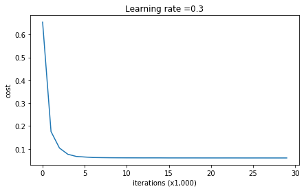
png
On the train set:
Accuracy: 0.928909952607
On the test set:
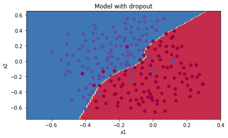
Accuracy: 0.951 | plt.title("Model with dropout") |
png
小结:
- 通过dropout操作,模型泛化性能得到大幅提升
- 一个常见错误是在训练和测试时都实施dropout操作,实际上,只需要在训练中使用
结论
- 正则化可以降低过拟合
- 正则化使得权系数变得更小
- L2正则化和dropout是两种非常有效的正则化手段
三种模型的结果对比
参考资料
- 吴恩达,coursera深度学习课程