神经网络的反向传播过程中,梯度计算十分重要。如果梯度计算有误,模型训练很难保证收敛。本文介绍一种验证梯度计算是否正确的方法,该方法简单有效,但是计算比较耗时,往往不会在每次训练过程中都进行验证,而是在需要确保梯度正确的时候才使用。
方法原理
求导(或梯度)的定义: \[ \frac{\partial J}{\partial \theta} = \lim_{\varepsilon \to 0} \frac{J(\theta + \varepsilon) - J(\theta - \varepsilon)}{2 \varepsilon} \tag{1}\]
已知条件:
- \(\frac{\partial J}{\partial \theta}\) 为待验证的目标.
- \(J\) 计算完全正确,可以计算 \(J(\theta + \varepsilon)\) 和 \(J(\theta - \varepsilon)\) (其中 \(\theta\) 为实数).
因此可以利用公式 (1) 和一个小量 \(\varepsilon\) 来验证 \(\frac{\partial J}{\partial \theta}\) 是正确的!
一维梯度验证
考虑一维线性函数 \(J(\theta) = \theta x\). 模型只包含一个实数参数 \(\theta\), \(x\) 为输入.
下面计算 \(J(.)\) 和它的导数 \(\frac{\partial J}{\partial \theta}\). 再验证 \(J\)的导数是正确的.
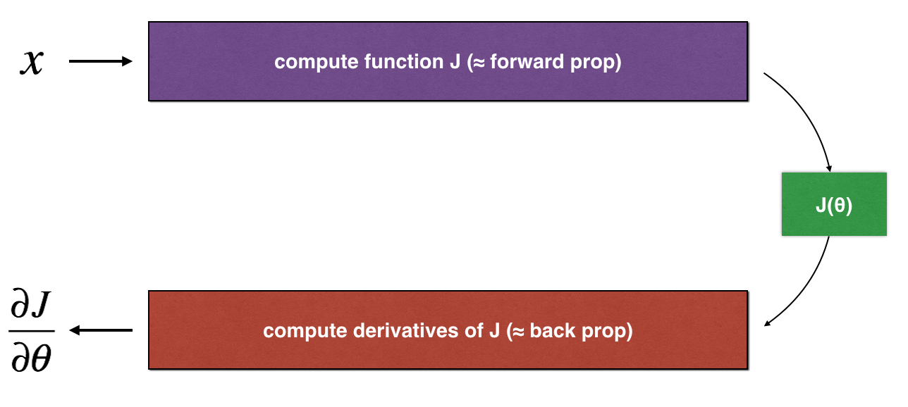
上图显示了关键的计算步骤: 首先输入 \(x\), 接着计算代价函数 \(J(x)\) ("正传"). 最后计算 \(\frac{\partial J}{\partial \theta}\) ("b反传").
1 | # Packages |
1 | # GRADED FUNCTION: forward_propagation |
1 | x, theta = 2, 4 |
J = 81 | # GRADED FUNCTION: backward_propagation |
1 | x, theta = 2, 4 |
dtheta = 2梯度验证步骤: - 首先利用公式(1)和一个小值 \(\varepsilon\)计算"gradapprox",具体的步骤包括: 1. \(\theta^{+} = \theta + \varepsilon\) 2. \(\theta^{-} = \theta - \varepsilon\) 3. \(J^{+} = J(\theta^{+})\) 4. \(J^{-} = J(\theta^{-})\) 5. \(gradapprox = \frac{J^{+} - J^{-}}{2 \varepsilon}\) - 利用反传函数计算 "grad" - 最后计算"gradapprox" 和"grad" 的差异: \[ difference = \frac {\mid\mid grad - gradapprox \mid\mid_2}{\mid\mid grad \mid\mid_2 + \mid\mid gradapprox \mid\mid_2} \tag{2}\] - 当差异很小时 (比如小于 \(10^{-7}\)), 则梯度计算正确,否则,梯度计算可能存在问题。
1 | # GRADED FUNCTION: gradient_check |
1 | x, theta = 2, 4 |
The gradient is correct!
difference = 2.91933588329e-10
N维梯度验证
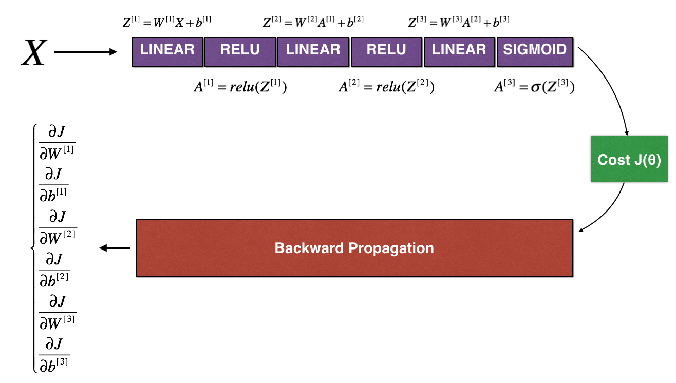
LINEAR -> RELU -> LINEAR -> RELU -> LINEAR -> SIGMOID
1 | def forward_propagation_n(X, Y, parameters): |
1 | def backward_propagation_n(X, Y, cache): |
梯度验证步骤:
和一维梯度验证类似,需要对比"gradapprox" 和反传函数计算的梯度:
\[ \frac{\partial J}{\partial \theta} = \lim_{\varepsilon \to 0} \frac{J(\theta + \varepsilon) - J(\theta - \varepsilon)}{2 \varepsilon} \tag{1}\]
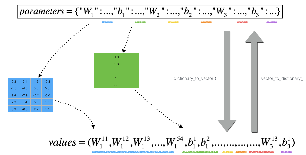
但是, \(\theta\) 不再是标量,而是一个字典"parameters". 此处提供了 "dictionary_to_vector()",它将字典 "parameters" 转化成向量 "values"。
逆过程为"vector_to_dictionary"输出字典 "parameters".
循环num_parameters个参数: - 计算J_plus[i]: 1. 令 \(\theta^{+}\) 为 np.copy(parameters_values) 2. 令 \(\theta^{+}_i\) 为 \(\theta^{+}_i + \varepsilon\) 3. 利用函数forward_propagation_n(x, y, vector_to_dictionary(\(\theta^{+}\) ))计算 \(J^{+}_i\) .
- 用相同的方法计算\(\theta^{-}\)的J_minus[i] - 计算 \(gradapprox[i] = \frac{J^{+}_i - J^{-}_i}{2 \varepsilon}\)
因此可以得到向量 gradapprox, 其中 gradapprox[i] 为相对于参数 parameter_values[i]的梯度近似结果. 将其对比反传函数计算的梯度向量. 和1D 情况下类似,计算: \[ difference = \frac {\| grad - gradapprox \|_2}{\| grad \|_2 + \| gradapprox \|_2 } \tag{3}\]
1 | # GRADED FUNCTION: gradient_check_n |
1 | X, Y, parameters = gradient_check_n_test_case() |
[93mThere is a mistake in the backward propagation! difference = 1.18904178788e-07[0m结论
- 梯度验证十分耗时,因此不会在训练的每一次迭代都进行梯度验证,而是只做几次验证
- 梯度验证不能和dropout一起使用,一般是在使用dropout之前保证梯度是正确的,然后再将dropout加进去
参考资料
- 吴恩达,coursera深度学习课程