在深度神经网络中采用一些先进的优化算法,不仅可以加速学习速度,还有可能获得更好的结果。本文介绍深度神经网络中最常用的三种优化算法:Mini-batch梯度下降法、动量法、Adam方法,并对一个简单数据集进行测试,对比三种方法的效果。
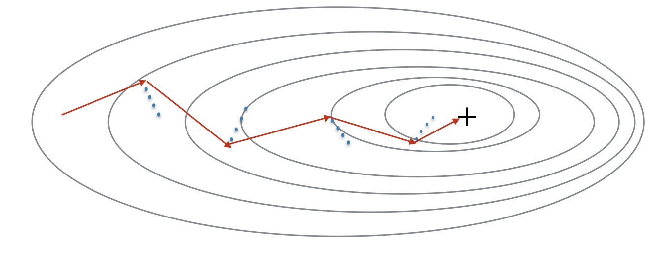
梯度下降法类似于以最快的方式寻找代价函数这座山的最低点: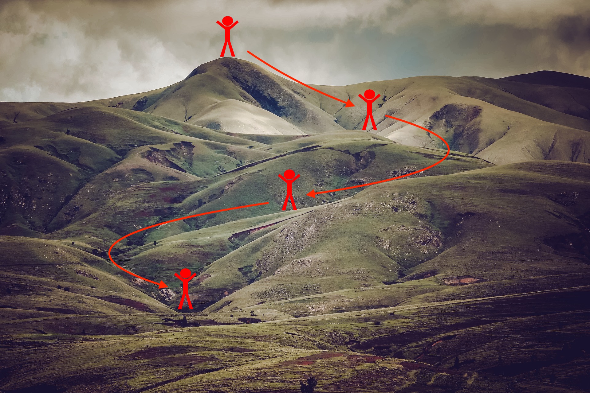
训练的每一步都是根据一定的方向更新参数,以可能走向最低的点.
标记: $ = $ da 对任意的 a.
1 | import numpy as np |
/media/seisinv/Data/svn/ai/learn/dl_ng/opt_utils.py:76: SyntaxWarning: assertion is always true, perhaps remove parentheses?
  assert(parameters['W' + str(l)].shape == layer_dims[l], layer_dims[l-1])
/media/seisinv/Data/svn/ai/learn/dl_ng/opt_utils.py:77: SyntaxWarning: assertion is always true, perhaps remove parentheses?
  assert(parameters['W' + str(l)].shape == layer_dims[l], 1)
梯度下降法
机器学习中最简单的优化方法是梯度下降法 (GD). 在每一步计算梯度过程中,如果使用所有m个样本, 该方法也称为 Batch Gradient Descent.
梯度下降准则: 对 \(l = 1, ..., L\): \[ W^{[l]} = W^{[l]} - \alpha \text{ } dW^{[l]} \tag{1}\] \[ b^{[l]} = b^{[l]} - \alpha \text{ } db^{[l]} \tag{2}\]
其中L 为层数, \(\alpha\) 为学习率. 所有的参数存储在字典 parameters 中。
1 | # GRADED FUNCTION: update_parameters_with_gd |
1 | parameters, grads, learning_rate = update_parameters_with_gd_test_case() |
W1 = [[ 1.63535156 -0.62320365 -0.53718766]
 [-1.07799357  0.85639907 -2.29470142]]
b1 = [[ 1.74604067]
 [-0.75184921]]
W2 = [[ 0.32171798 -0.25467393  1.46902454]
 [-2.05617317 -0.31554548 -0.3756023 ]
 [ 1.1404819  -1.09976462 -0.1612551 ]]
b2 = [[-0.88020257]
 [ 0.02561572]
[ 0.57539477]]另一个变种是随机梯度下降法,相当于min-batch=1个样本的mini-batch GD方法。
- (Batch) Gradient Descent:
1 | X = data_input |
- Stochastic Gradient Descent:
1 | X = data_input |
在随机梯度下降法中,每次更新梯度只用一个训练样本,当训练集很大时,SGD会更快,但是参数更新过程会十分震荡,而不会平滑收敛。
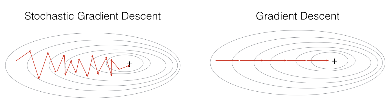
"+" 表示代价函数的最低点. SGD 震荡剧烈直到收敛. 但是,由于 SGD只用一个样本而不是所有样本计算梯度,因此它的每一步要远快于GD.
SGD实现过程有3个循环: 1. 迭代循环Over the number of iterations 2. \(m\)个样本循环 3. 层数循环 (以更新所有参数, 从 \((W^{[1]},b^{[1]})\) 到 \((W^{[L]},b^{[L]})\))
相比较而言,Mini-batch gradient descent 每一步使用一部分样本. 不需要对每个样本循环,而是对每个batch循环. 这样不仅减少震荡,而且可以利用python的向量化特点,加快收敛速度。
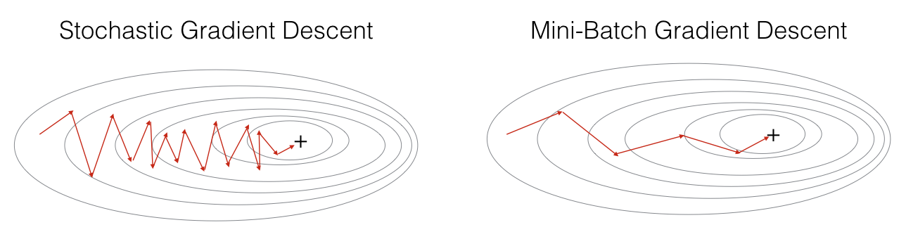
"+" 表示代价函数的最低点. 利用 mini-batches 往往是最快的优化方式.
小结: - gradient descent, mini-batch gradient descent and stochastic gradient descent的差异在于每次模型更新所用的样本个数. - mini-batch需要不停调整. - 使用合理的 mini-batch 大小, mini-batch方法往往由于gradient descent 和 stochastic gradient descent 方法(尤其是当训练集很大的情况).
Mini-Batch 梯度下降法
从训练集(X, Y)建立mini-batches可以分两步:
- Shuffle: 建立训练集的 shuffled 版本,如下图所示. X 和 Y 每一列代表一个训练样本. 注意是同时对X 和 Y进行随机 shuffling. 这样才能保证shuffling 之后X的第 \(i^{th}\)X 和Y的 \(i^{th}\) 仍然是对应起来的. shuffling 使得样本是随机分割成不同的mini-batches.
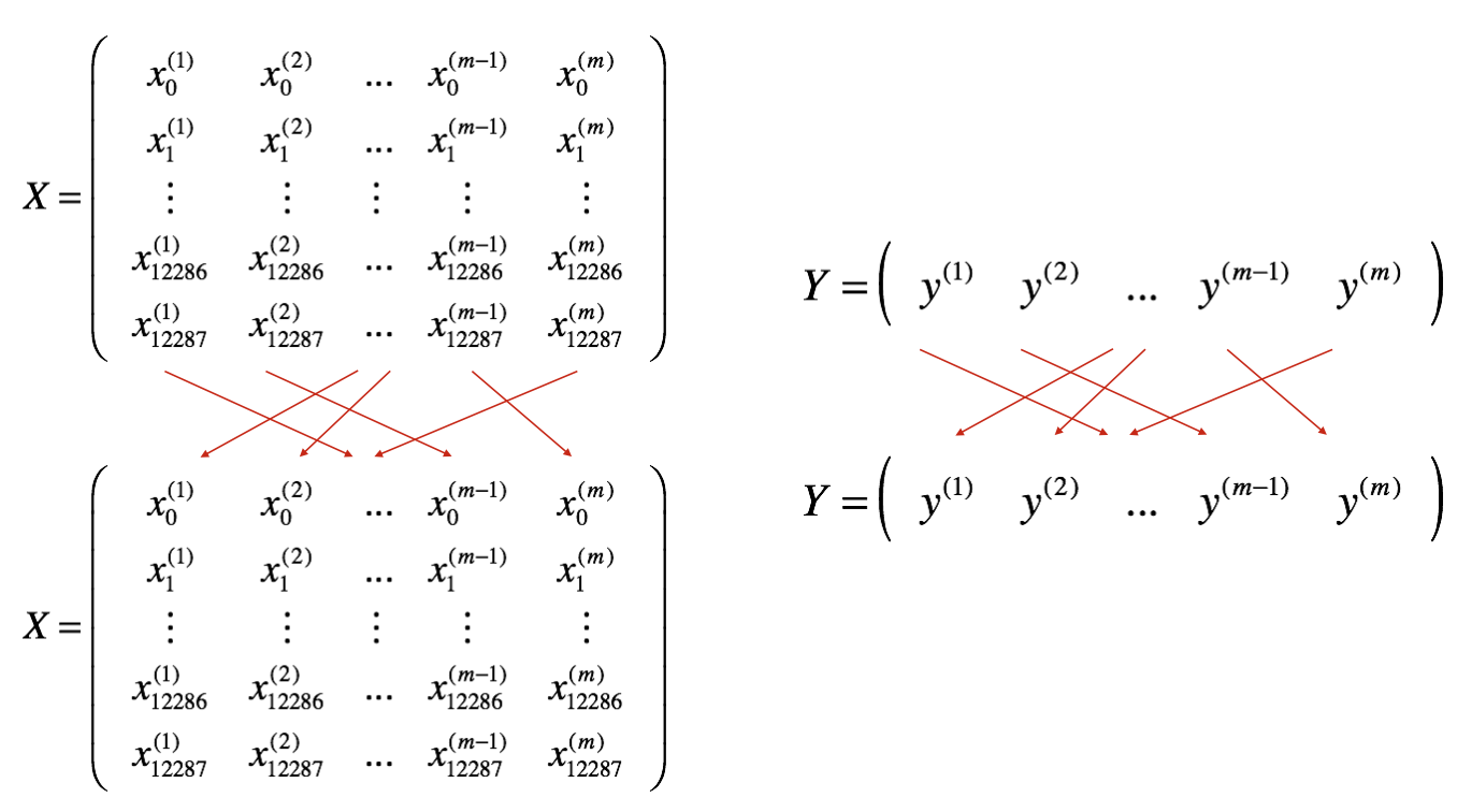
- Partition: 将shuffled之后的(X, Y) 分割成大小为
mini_batch_size(here 64)的mini-batches. 注意训练样本不一定可以整除mini_batch_size. 最后的mini-batche可能比较小, 当它小于完整的mini_batch_size时:

实现了Shuffle之后,选择第1和第2个mini-batches的代码为: 1
2
3first_mini_batch_X = shuffled_X[:, 0 : mini_batch_size]
second_mini_batch_X = shuffled_X[:, mini_batch_size : 2 * mini_batch_size]
...
注意到最后的min-batch可能小于mini_batch_size=64. 令 \(\lfloor s \rfloor\) 表示 对\(s\) 不大于它的整数 (也就是python中的 math.floor(s)). 如果总样本数不是mini_batch_size=64的乘积,那么会有 \(\lfloor \frac{m}{mini\_batch\_size}\rfloor\) 个64 样本的mini-batch, 而最后的mini-batch 大小为 (\(m-mini_\_batch_\_size \times \lfloor \frac{m}{mini\_batch\_size}\rfloor\)).
1 | # GRADED FUNCTION: random_mini_batches |
1 | X_assess, Y_assess, mini_batch_size = random_mini_batches_test_case() |
shape of the 1st mini_batch_X: (12288, 64)
shape of the 2nd mini_batch_X: (12288, 64)
shape of the 3rd mini_batch_X: (12288, 20)
shape of the 1st mini_batch_Y: (1, 64)
shape of the 2nd mini_batch_Y: (1, 64)
shape of the 3rd mini_batch_Y: (1, 20)
mini batch sanity check: [ 0.90085595 -0.7612069 0.2344157 ]小结:
- Shuffling 和 Partitioning 是生成min-batch的两步
- 2的次方往往选做min-batch的大小,如16,32,64,128d.
动量
由于mini-batch梯度下降法每次参数更新都仅仅用了一部分数据,因此更新方向会有一些震荡。采用动量可以减少这种震荡。
动量策略考虑了以前的梯度信息以对更新量进行平滑处理。之前的梯度方向会存在变量 \(v\)中。更准确的说,\(v\)是之前梯度的指数加权平均。也可以把\(v\)看做球往山下滚的速度,新计算的梯度作为动量修正\(v\).
动量更新, 循环 \(l = 1, ..., L\):
\[ \begin{cases} v_{dW^{[l]}} = \beta v_{dW^{[l]}} + (1 - \beta) dW^{[l]} \\ W^{[l]} = W^{[l]} - \alpha v_{dW^{[l]}} \end{cases}\tag{3}\]
\[\begin{cases} v_{db^{[l]}} = \beta v_{db^{[l]}} + (1 - \beta) db^{[l]} \\ b^{[l]} = b^{[l]} - \alpha v_{db^{[l]}} \end{cases}\tag{4}\]
其中 L 为层数, \(\beta\) 为动量, \(\alpha\)为学习率.
1 | # GRADED FUNCTION: initialize_velocity |
1 | parameters = initialize_velocity_test_case() |
v["dW1"] = [[ 0.  0.  0.]
 [ 0.  0.  0.]]
v["db1"] = [[ 0.]
 [ 0.]]
v["dW2"] = [[ 0.  0.  0.]
 [ 0.  0.  0.]
 [ 0.  0.  0.]]
v["db2"] = [[ 0.]
 [ 0.]
 [ 0.]]
1 | # GRADED FUNCTION: update_parameters_with_momentum |
1 | parameters, grads, v = update_parameters_with_momentum_test_case() |
W1 = [[ 1.62544598 -0.61290114 -0.52907334]
 [-1.07347112  0.86450677 -2.30085497]]
b1 = [[ 1.74493465]
 [-0.76027113]]
W2 = [[ 0.31930698 -0.24990073  1.4627996 ]
 [-2.05974396 -0.32173003 -0.38320915]
 [ 1.13444069 -1.0998786  -0.1713109 ]]
b2 = [[-0.87809283]
 [ 0.04055394]
 [ 0.58207317]]
v["dW1"] = [[-0.11006192  0.11447237  0.09015907]
 [ 0.05024943  0.09008559 -0.06837279]]
v["db1"] = [[-0.01228902]
 [-0.09357694]]
v["dW2"] = [[-0.02678881  0.05303555 -0.06916608]
 [-0.03967535 -0.06871727 -0.08452056]
 [-0.06712461 -0.00126646 -0.11173103]]
v["db2"] = [[ 0.02344157]
 [ 0.16598022]
[ 0.07420442]]如何选择\(\beta\):
- \(\beta\)越大,则考虑更多以前的梯度,更新越平滑,如果过大,会导平滑掉有效更新量
- \(\beta\)常见的取值范围从0.8到0.999,如果不想调这个参数,\(\beta=0.9\)往往是一个合理的选择
小结:
- 动量方法考虑之前的梯度信息,以平滑梯度下降法的搜索方向,可以应用在batch GD, mini-batch GD和随机GD方法中
- 增加了一个超级参数\(\beta\)需要调整
Adam方法
Adam方法是神经网络中最有效的优化算法,它结合了RMSProp和动量两种方法的思想。
Adam 工作原理 1. 计算之前梯度的指数加权平均,并保存在变量\(v\)中 (偏差校正前) 和 \(v^{corrected}\) (偏差校正后). 2. 计算之前梯度平方的指数加权平均,并保存在变量\(s\)中 (偏差校正前) 和 \(s^{corrected}\) (偏差校正后). 3. 结合步骤 "1" 和 "2"得到新的更新方向,对模型进行更新.
更新准则是, 循环 \(l = 1, ..., L\):
\[\begin{cases}
v_{dW^{[l]}} = \beta_1 v_{dW^{[l]}} + (1 - \beta_1) \frac{\partial \mathcal{J} }{ \partial W^{[l]} } \\
v^{corrected}_{dW^{[l]}} = \frac{v_{dW^{[l]}}}{1 - (\beta_1)^t} \\
s_{dW^{[l]}} = \beta_2 s_{dW^{[l]}} + (1 - \beta_2) (\frac{\partial \mathcal{J} }{\partial W^{[l]} })^2 \\
s^{corrected}_{dW^{[l]}} = \frac{s_{dW^{[l]}}}{1 - (\beta_1)^t} \\
W^{[l]} = W^{[l]} - \alpha \frac{v^{corrected}_{dW^{[l]}}}{\sqrt{s^{corrected}_{dW^{[l]}}} + \varepsilon}
\end{cases}\] 其中: - t 计算Adam的步数
- L 层数
- \(\beta_1\) 和 \(\beta_2\) 为控制两个指数加权平均的超参
- \(\alpha\) 为学习率
- \(\varepsilon\) 避免除0的小值
1 | # GRADED FUNCTION: initialize_adam |
1 | parameters = initialize_adam_test_case() |
v["dW1"] = [[ 0.  0.  0.]
 [ 0.  0.  0.]]
v["db1"] = [[ 0.]
 [ 0.]]
v["dW2"] = [[ 0.  0.  0.]
 [ 0.  0.  0.]
 [ 0.  0.  0.]]
v["db2"] = [[ 0.]
 [ 0.]
 [ 0.]]
s["dW1"] = [[ 0.  0.  0.]
 [ 0.  0.  0.]]
s["db1"] = [[ 0.]
 [ 0.]]
s["dW2"] = [[ 0.  0.  0.]
 [ 0.  0.  0.]
 [ 0.  0.  0.]]
s["db2"] = [[ 0.]
 [ 0.]
 [ 0.]]
1 | # GRADED FUNCTION: update_parameters_with_adam |
1 | parameters, grads, v, s = update_parameters_with_adam_test_case() |
W1 = [[ 1.63178673 -0.61919778 -0.53561312]
 [-1.08040999  0.85796626 -2.29409733]]
b1 = [[ 1.75225313]
 [-0.75376553]]
W2 = [[ 0.32648046 -0.25681174  1.46954931]
 [-2.05269934 -0.31497584 -0.37661299]
 [ 1.14121081 -1.09245036 -0.16498684]]
b2 = [[-0.88529978]
 [ 0.03477238]
 [ 0.57537385]]
v["dW1"] = [[-0.11006192  0.11447237  0.09015907]
 [ 0.05024943  0.09008559 -0.06837279]]
v["db1"] = [[-0.01228902]
 [-0.09357694]]
v["dW2"] = [[-0.02678881  0.05303555 -0.06916608]
 [-0.03967535 -0.06871727 -0.08452056]
 [-0.06712461 -0.00126646 -0.11173103]]
v["db2"] = [[ 0.02344157]
 [ 0.16598022]
 [ 0.07420442]]
s["dW1"] = [[ 0.00121136  0.00131039  0.00081287]
 [ 0.0002525   0.00081154  0.00046748]]
s["db1"] = [[  1.51020075e-05]
 [  8.75664434e-04]]
s["dW2"] = [[  7.17640232e-05   2.81276921e-04   4.78394595e-04]
 [  1.57413361e-04   4.72206320e-04   7.14372576e-04]
 [  4.50571368e-04   1.60392066e-07   1.24838242e-03]]
s["db2"] = [[  5.49507194e-05]
 [  2.75494327e-03]
 [  5.50629536e-04]]
测试不同的优化算法
1 | train_X, train_Y = load_dataset() |

png
1 | def model(X, Y, layers_dims, optimizer, learning_rate = 0.0007, mini_batch_size = 64, beta = 0.9, |
Mini-batch梯度下降法
1 | # train 3-layer model |
Cost after epoch 0: 0.690736
Cost after epoch 1000: 0.685273
Cost after epoch 2000: 0.647072
Cost after epoch 3000: 0.619525
Cost after epoch 4000: 0.576584
Cost after epoch 5000: 0.607243
Cost after epoch 6000: 0.529403
Cost after epoch 7000: 0.460768
Cost after epoch 8000: 0.465586
Cost after epoch 9000: 0.464518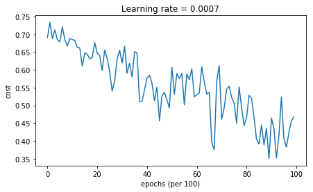
png
Accuracy: 0.796666666667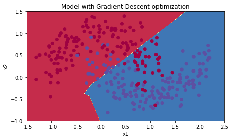
png
带动量的Mini-batch梯度下降法
1 | # train 3-layer model |
Cost after epoch 0: 0.690741
Cost after epoch 1000: 0.685341
Cost after epoch 2000: 0.647145
Cost after epoch 3000: 0.619594
Cost after epoch 4000: 0.576665
Cost after epoch 5000: 0.607324
Cost after epoch 6000: 0.529476
Cost after epoch 7000: 0.460936
Cost after epoch 8000: 0.465780
Cost after epoch 9000: 0.464740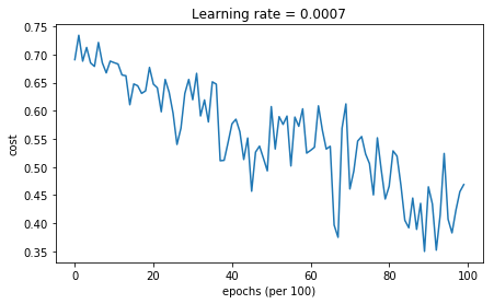
png
Accuracy: 0.796666666667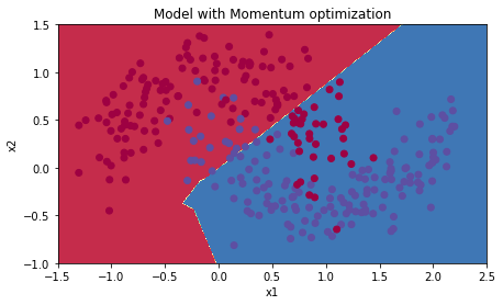
png
Adam模式下的Mini-batch梯度下降法
1 | # train 3-layer model |
Cost after epoch 0: 0.690552
Cost after epoch 1000: 0.185501
Cost after epoch 2000: 0.150830
Cost after epoch 3000: 0.074454
Cost after epoch 4000: 0.125959
Cost after epoch 5000: 0.104344
Cost after epoch 6000: 0.100676
Cost after epoch 7000: 0.031652
Cost after epoch 8000: 0.111973
Cost after epoch 9000: 0.197940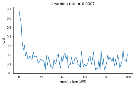
png
Accuracy: 0.94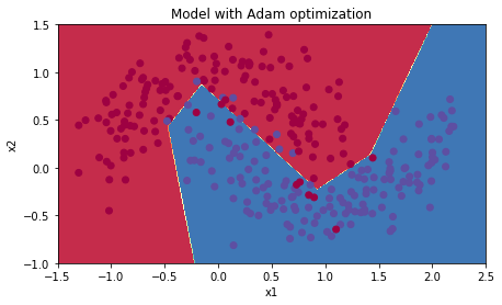
png
结论
- 动量法往往有帮助,但是对于小的学习率和简单数据集,影响几乎可以忽略。
- 代价函数的剧烈波动来自于对优化算法来说,一些minibatch更加复制。
- Adam方法明显优于min-batch梯度下降法和动量法,但是如果给予足够的迭代次数,所有三种方法的结果会类似。但是,Adam方法收敛速度快得多。
- Adam方法的优点包括:仅需要很小的内存;往往不需要调参就可以工作很好(学习率除外)。
参考资料
- 吴恩达,coursera深度学习课程