本文介绍一种十分通用的深度学习编程框架:Tensorflow。该变成框架主要包含两个对象:张量和操作。通过这两个对象可以建立一个计算图,再启动会话以执行该计算图。对深度神经网络应用来说,只需要在会话中运行“optimizer”对象,Tensoflow就可以自动运行反传和模型更新,十分便捷。
基本用法
对单个样本,计算代价函数: \[loss = \mathcal{L}(\hat{y}, y) = (\hat y^{(i)} - y^{(i)})^2 \tag{1}\]
1 | import math |
1 | y_hat = tf.constant(36, name='y_hat') # Define y_hat constant. Set to 36. |
9在Tensorflow下编写和运行程序有以下几步:
- 建立张量或变量
- 编写张量之间的操作
- 初始化张量
- 建立一个session
- 运行这个session,此时会执行前面编写的操作
1 | a = tf.constant(2) |
Tensor("Mul:0", shape=(), dtype=int32)从上面可以看出,你并没有看到20,而是输出一个没有维度信息的张量。上面的语句只是把操作放进了“运算图”中,并没有执行运算。为了执行运算,需要建立一个session,然后运行这个session。
1 | sess = tf.Session() |
20下面介绍placeholder的用法,placeholder是一个对象,它的值可以稍后指定。为了对这个placeholder设定值,可以使用"feed dictionary"(变量feed_dict)。下面是一个简单的例子:
1 | # Change the value of x in the feed_dict |
6线性函数
计算 \(Y = WX + b\), 其中 \(W\) 和 \(X\) 都是随机向量
1 | # GRADED FUNCTION: linear_function |
1 | print( "result = " + str(linear_function())) |
result = [[-2.15657382]
 [ 2.95891446]
 [-1.08926781]
 [-0.84538042]]
计算sigmoid函数
1 | # GRADED FUNCTION: sigmoid |
1 | print ("sigmoid(0) = " + str(sigmoid(0))) |
sigmoid(0) = 0.5
sigmoid(12) = 0.999994
计算代价函数
对2层神经网络,代价函数是 \(a^{[2](i)}\) 和 \(y^{(i)}\)的函数, for i=1...m: \[ J = - \frac{1}{m} \sum_{i = 1}^m \large ( \small y^{(i)} \log a^{ [2] (i)} + (1-y^{(i)})\log (1-a^{ [2] (i)} )\large )\small\tag{2}\]
Tensoflow只需要一行代码 - tf.nn.sigmoid_cross_entropy_with_logits(logits = ..., labels = ...) 计算的是: \[- \frac{1}{m} \sum_{i = 1}^m \large ( \small y^{(i)} \log \sigma(z^{[2](i)}) + (1-y^{(i)})\log (1-\sigma(z^{[2](i)})\large )\small\tag{2}\]
1 | # GRADED FUNCTION: cost |
1 | logits = sigmoid(np.array([0.2,0.4,0.7,0.9])) |
cost = [ 1.00538719 1.03664088 0.41385433 0.39956614]One Hot编码
在深度学习中,经常会有向量y从 0 到 C-1变化, 其中 C 是类别数.如果C 为4的话,需要转化成下面的形式::
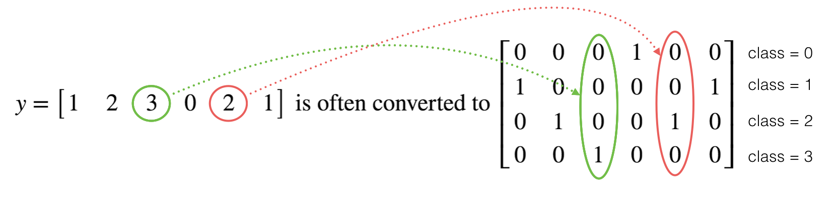
上面称为"one hot" 编码, 这个名字起源于每一列只有一个元素是热点(为1). 为实现这个功能,numpy可能需要几行代码,而tensorflow只需要一行,:
- tf.one_hot(labels, depth, axis)
1 | # GRADED FUNCTION: one_hot_matrix |
1 | labels = np.array([1,2,3,0,2,1]) |
one_hot = [[ 0.  0.  0.  1.  0.  0.]
 [ 1.  0.  0.  0.  0.  1.]
 [ 0.  1.  0.  0.  1.  0.]
 [ 0.  0.  1.  0.  0.  0.]]
初始化0和1
1 | # GRADED FUNCTION: ones |
1 | print ("ones = " + str(ones([3]))) |
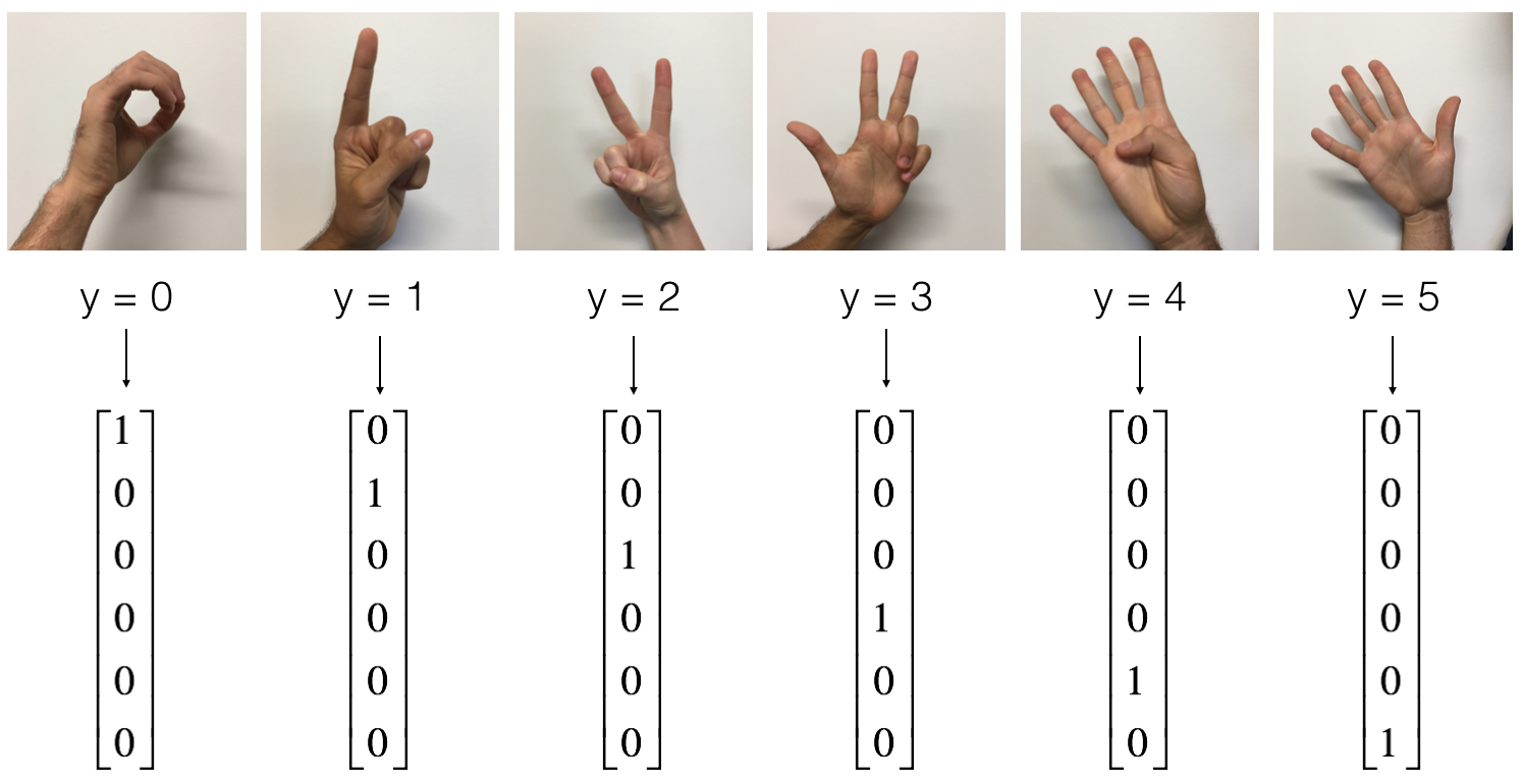
ones = [ 1. 1. 1.]建立第一个神经网络
- 训练集: 1080 张代表0-5的图 (64 × 64) (每个数字180 张图).
- 测试集: 120 张代表0-5的图 (64 × 64 )(每个数字20 张图).
1 | # Loading the dataset |
1 | # Example of a picture |
y = 5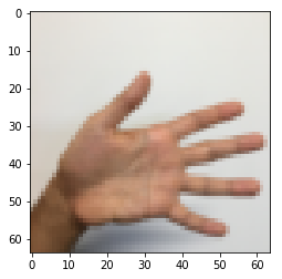
png
1 | # Flatten the training and test images |
number of training examples = 1080
number of test examples = 120
X_train shape: (12288, 1080)
Y_train shape: (6, 1080)
X_test shape: (12288, 120)
Y_test shape: (6, 120)模型:LINEAR -> RELU -> LINEAR -> RELU -> LINEAR -> SOFTMAX. 与二分类使用 SIGMOID 作为输出层不同, 多分类问题使用 SOFTMAX.
建立占位符
首先建立X和Y的占位符,然后在运行会话时,将训练数据集传进占位符。
1 | # GRADED FUNCTION: create_placeholders |
1 | X, Y = create_placeholders(12288, 6) |
X = Tensor("X_1:0", shape=(12288, ?), dtype=float32)
Y = Tensor("Y:0", shape=(6, ?), dtype=float32)
参数初始化
采用Xavier初始化权系数,零初始化偏置量
1 | # GRADED FUNCTION: initialize_parameters |
1 | tf.reset_default_graph() |
W1 = <tf.Variable 'W1:0' shape=(25, 12288) dtype=float32_ref>
b1 = <tf.Variable 'b1:0' shape=(25, 1) dtype=float32_ref>
W2 = <tf.Variable 'W2:0' shape=(12, 25) dtype=float32_ref>
b2 = <tf.Variable 'b2:0' shape=(12, 1) dtype=float32_ref>
正传播
需要注意的是,和之前使用numpy实现正传不同,tensorflow的线性层最终输出为z3,这是因为最后要使用z3作为输入计算代价函数,所以不需要提前计算a3。
1 | # GRADED FUNCTION: forward_propagation |
1 | tf.reset_default_graph() |
Z3 = Tensor("Add_2:0", shape=(6, ?), dtype=float32)计算代价函数
需要注意的是,tensorflow中只需要一行代码计算: 1
tf.reduce_mean(tf.nn.softmax_cross_entropy_with_logits(logits = ..., labels = ...))
但是需要"logits" 和 "labels"的输入维度是(样本数, 分类数)。另外tf.reduce_mean是对所有样本求和。
1 | # GRADED FUNCTION: compute_cost |
1 | tf.reset_default_graph() |
cost = Tensor("Mean:0", shape=(), dtype=float32)反传及参数更新
这是使用编程框架的优势所在,所有的反传和模型更新只需要几行代码。
计算代价函数之后,就可以建立一个“优化”对象。在会话开始运行之后,调用这个对象,就会根据选择的优化方法和学习率优化这个目标函数
例如,使用梯度下降法: 1
optimizer = tf.train.GradientDescentOptimizer(learning_rate = learning_rate).minimize(cost)
运行优化算法: 1
_ , c = sess.run([optimizer, cost], feed_dict={X: minibatch_X, Y: minibatch_Y})
上面的语句则会实现反传及参数更新。
建立模型
1 | def model(X_train, Y_train, X_test, Y_test, learning_rate = 0.0001, |
1 | parameters = model(X_train, Y_train, X_test, Y_test) |
Cost after epoch 0: 1.855702
Cost after epoch 100: 1.016458
Cost after epoch 200: 0.733102
Cost after epoch 300: 0.572940
Cost after epoch 400: 0.468774
Cost after epoch 500: 0.381021
Cost after epoch 600: 0.313822
Cost after epoch 700: 0.254158
Cost after epoch 800: 0.203829
Cost after epoch 900: 0.166421
Cost after epoch 1000: 0.141486
Cost after epoch 1100: 0.107580
Cost after epoch 1200: 0.086270
Cost after epoch 1300: 0.059371
Cost after epoch 1400: 0.052228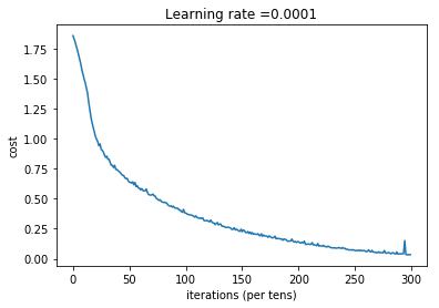
png
Parameters have been trained!
Train Accuracy: 0.999074
Test Accuracy: 0.716667小结:模型过拟合,可以采用L2正则化或者dropout方法缓解过拟合问题
测试用户的图像
1 | import scipy |
Your algorithm predicts: y = 3
png
小结:上面的测试数据分类错误,这是因为训练数据集中没有这样的数据,于是出现了数据分布不匹配的问题。这是深度学习中一个非常经典的问题。
结论
- Tensorflow是一种广泛使用的深度学习编程框架,它主要包含两个对象类:张量和操作
- 使用Tensorflow必须遵循这样几步:
- 建立计算图,包括张量(变量、占位符等)和操作(加法、乘法等)
- 建立一个会话
- 初始化会话
- 运行会话以执行计算图
- 计算图可以执行多次,如model()函数所示
- 在Tensorflow中,当运行“optimizer”对象之后,反传和模型更新是自动运行的。
参考资料
- 吴恩达,coursera深度学习课程