本文将介绍卷积神经网络的基本原理,以及如何利用numpy库函数搭建CNN,包括实现卷积层、POOL层以及对应的正传和反传。
符号 - 上标 \([l]\) 代表第 \(l\) 层的数值.
- 例如: \(a^{[L]}\) 表示第 \(L\) 层激活函数的输出. \(W^{[L]}\) 和 \(b^{[L]}\) 表示第 \(L\) 层的参数.
- 上标 \((i)\) 表示第 \(i\) 样本.
- 例如: \(x^{(i)}\) 表示第 \(i\) 训练样本.
- 下标 \(i\) 表示向量的第 \(i\) 个元素.
- 例如: \(a^{[l]}_i\) 表示第\(l\)层第\(i\)个神经元的输出.
- \(n_H\), \(n_W\) 和 \(n_C\) 分别表示给定层的高、宽和深度. 如果指定层\(l\), 则高、宽、深度为 \(n_H^{[l]}\), \(n_W^{[l]}\), \(n_C^{[l]}\).
- \(n_{H_{prev}}\), \(n_{W_{prev}}\) 和 \(n_{C_{prev}}\) 分别表示上一层的高、宽和深度,如果参考层为 \(l\), 则为 \(n_H^{[l-1]}\), \(n_W^{[l-1]}\), \(n_C^{[l-1]}\).
本文将要实现的模型如下:
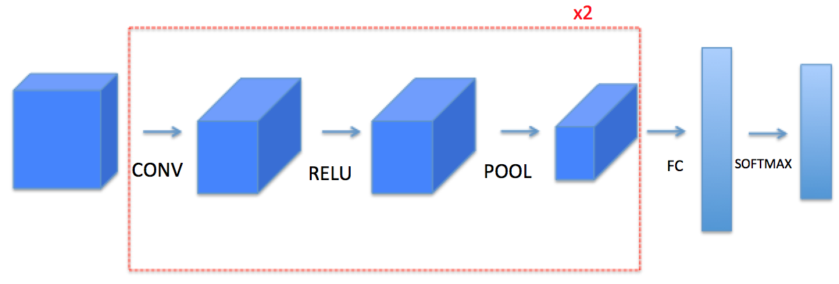
卷积神经网络
卷积层是CNN中最难理解的一个概念,它将输入体转化成不同大小的输出体,如图所示:
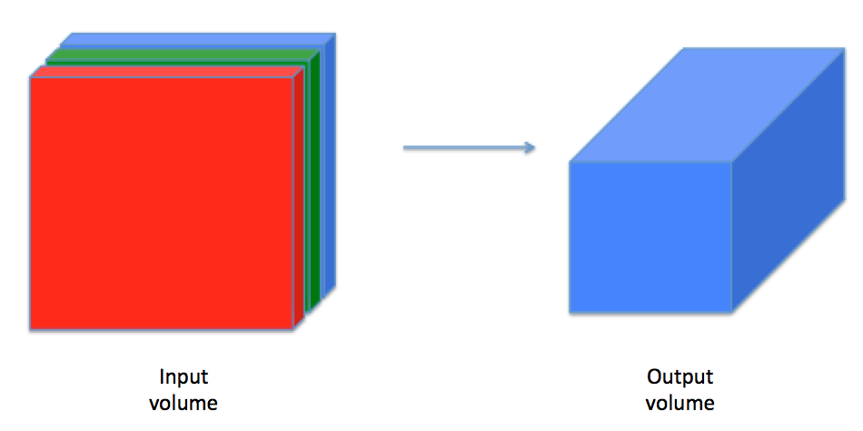
下面将介绍卷基层中的两个基本元素:补零和卷积
补零
补零是指在图像边界增加0元素。

图像 (3 通道, RGB) 补2个零元素.
补零的主要好处有:
- 保证卷基层的高和宽不变。如果不补零,随着深度的增加,输出的高和宽会越来越小。补零的一个特殊补法叫“SAME”,意思是补零以保证卷积前后高和宽保持不变。
- 保留更多图像边界的信息。如果不补零,图像边界的信息对下一层的影响很小。
在numpy中,对一个形状为(5,5,5,5,5)的数组第1和第2维度两端分别补1和3个零,函数是:
1 | a = np.pad(a, ((0,0), (1,1), (0,0), (3,3), (0,0)), 'constant', constant_values = (..,..)) |
1 | import numpy as np |
1 | # GRADED FUNCTION: zero_pad |
1 | np.random.seed(1) |
x.shape = (4, 3, 3, 2)
x_pad.shape = (4, 7, 7, 2)
x[1, 1] = [[ 0.90085595 -0.68372786]
 [-0.12289023 -0.93576943]
 [-0.26788808  0.53035547]]
x_pad[1, 1] = [[ 0.  0.]
 [ 0.  0.]
 [ 0.  0.]
 [ 0.  0.]
 [ 0.  0.]
 [ 0.  0.]
 [ 0.  0.]]


<matplotlib.image.AxesImage at 0x7fb7094a0860>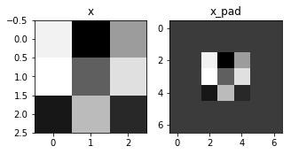
png
卷积操作
卷积每一步每一步操作是将一个滤波器应用在输入图像的一个特定位置,包括:
- 输入图像
- 对图像的每个位置应用这个滤波器
- 输入结果(通常大小发生变化)

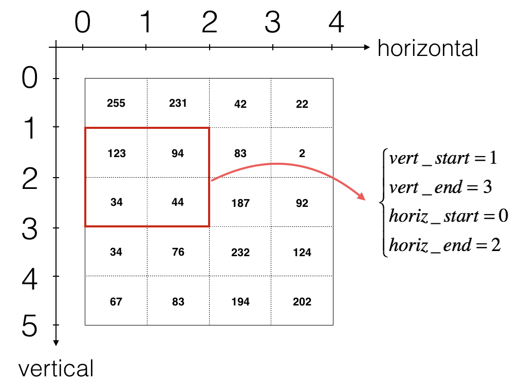
应用步长为1 大小为2x2 的滤波器 (步长 = 每次移动窗口的大小)
在计算机视觉中,左边矩阵的每一个元素为一个像素点。对左边矩阵应用一个33滤波器进行卷积操作,意味着从该矩阵中取出33大小的元素和这个滤波器点点对应相乘,然后求和。
1 | # GRADED FUNCTION: conv_single_step |
1 | np.random.seed(1) |
Z = -23.1602122025正传
在正传播过程,每次应用“卷积”就输出一个2D矩阵,多次应用不同的滤波器,叠加起来就形成一个三维体。
本图只展示一个通道的情况.
卷积前后维度变化公式:
\[ n_H = \lfloor \frac{n_{H_{prev}} - f + 2 \times pad}{stride} \rfloor +1 \] \[ n_W = \lfloor \frac{n_{W_{prev}} - f + 2 \times pad}{stride} \rfloor +1 \] \[ n_C = \text{使用的滤波器个数}\]
1 | # GRADED FUNCTION: conv_forward |
1 | np.random.seed(1) |
Z's mean = 0.155859324889
cache_conv[0][1][2][3] = [-0.20075807  0.18656139  0.41005165]
最后,卷基层可以再增加一个激活函数:
1 | # Convolve the window to get back one output neuron |
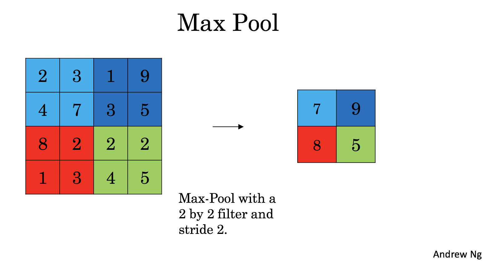
池化层
池化层 (POOL) 减少输入数据的高度和宽度,有利于减少计算量,也有利于使得特征检测与输入数据的位置更加无关. 有两种池化方法:
最大池化层: 在输入图像上移动一个 (\(f, f\)) 窗口,输出这个窗口内的最大值.
平均池化层: 在输入图像上移动一个 (\(f, f\)) 窗口,输出这个窗口内的平均值.
|

|
池化层没有参数需要训练,但是有超参(例如窗口大小f)需要调整。.
正向池化
分别实现 MAX-POOL 和 AVG-POOL.
池化前后数据的维度变化: \[ n_H = \lfloor \frac{n_{H_{prev}} - f}{stride} \rfloor +1 \] \[ n_W = \lfloor \frac{n_{W_{prev}} - f}{stride} \rfloor +1 \] \[ n_C = n_{C_{prev}}\] 注意池化前一般不会补零;池化也不会变化输入输出数据的深度
1 | # GRADED FUNCTION: pool_forward |
1 | np.random.seed(1) |
mode = max
A = [[[[ 1.74481176  1.6924546   2.10025514]]]


 [[[ 1.19891788  1.51981682  2.18557541]]]]

mode = average
A = [[[[-0.09498456  0.11180064 -0.14263511]]]


 [[[-0.09525108  0.28325018  0.33035185]]]]
卷基层反向传播
当前深度学习框架中,往往只需要实现正向传播,编程框架会自动实现反向传播。但是也有必要了解反向传播的工作原理。
反向卷积操作
计算dA
对于一个特定的滤波器\(W_c\)和一个特定的训练样本,\(dA\)的表达式:
\[ dA += \sum _{h=0} ^{n_H} \sum_{w=0} ^{n_W} W_c \times dZ_{hw} \tag{1}\]
其中 \(W_c\) 为一个滤波器 \(dZ_{hw}\) 为代价函数关于卷积层在第h行、第w列的输出Z的梯度。注意上面的公式,每次对不同的dZ乘以相同的\(W_c\)。 在正传过程中,每个旅欧波器点乘不同的切片并求和,因此,在反传时,将所有切片的提取求和。
上面的公式转化为代码为: 1
da_prev_pad[vert_start:vert_end, horiz_start:horiz_end, :] += W[:,:,:,c] * dZ[i, h, w, c]
计算 dW
计算 \(dW_c\) (\(dW_c\) 是代价函数关于一个滤波器的梯度):
\[ dW_c += \sum _{h=0} ^{n_H} \sum_{w=0} ^ {n_W} a_{slice} \times dZ_{hw} \tag{2}\]
其中 \(a_{slice}\) 用于生成激励 \(Z_{ij}\)的切片. 因此, 公式提供了关于这个切片的 \(W\)梯度 . 由于所有的滤波器 \(W\)相同, 因此将所有的梯度求和得到\(dW\).
对应的代码为: 1
dW[:,:,:,c] += a_slice * dZ[i, h, w, c]
计算 db:
对一个特定滤波器 \(W_c\),关于该代价函数计算\(db\)的公式为:
\[ db = \sum_h \sum_w dZ_{hw} \tag{3}\]
对应的代码为: 1
db[:,:,:,c] += dZ[i, h, w, c]
1 | def conv_backward(dZ, cache): |
1 | np.random.seed(1) |
dA_mean = 9.60899067587
dW_mean = 10.5817412755
db_mean = 76.3710691956
池化层反传
最大池化层反传
首先建立函数create_mask_from_window() 实现:
\[ X = \begin{bmatrix} 1 && 3 \\ 4 && 2 \end{bmatrix} \quad \rightarrow \quad M =\begin{bmatrix} 0 && 0 \\ 1 && 0 \end{bmatrix}\tag{4}\]
该函数标记了输入层中对输出有影响的位置。
1 | def create_mask_from_window(x): |
1 | np.random.seed(1) |
x =  [[ 1.62434536 -0.61175641 -0.52817175]
 [-1.07296862  0.86540763 -2.3015387 ]]
mask =  [[ True False False]
 [False False False]]
平均池化反传
为了描述平均池化层中输入数据对输出数据的影响,建立函数实现:
\[ dZ = 1 \quad \rightarrow \quad dZ =\begin{bmatrix} 1/4 && 1/4 \\ 1/4 && 1/4 \end{bmatrix}\tag{5}\]
1 | def distribute_value(dz, shape): |
1 | a = distribute_value(2, (2,2)) |
distributed value = [[ 0.5  0.5]
 [ 0.5  0.5]]
池化层反传
1 | def pool_backward(dA, cache, mode = "max"): |
1 | np.random.seed(1) |
mode = max
mean of dA =  0.145713902729
dA_prev[1,1] =  [[ 0.          0.        ]
 [ 5.05844394 -1.68282702]
 [ 0.          0.        ]]

mode = average
mean of dA =  0.145713902729
dA_prev[1,1] =  [[-0.32345834  0.45074345]
 [ 2.52832571 -0.24863478]
 [ 1.26416285 -0.12431739]]
结论
- 本文介绍CNN的基本原理,以及实现卷基层各个构成部分
- 反传部分有助于进一步理解CNN的工作机理,但是在主流的深度学习框架中,都不需要自己实现,而只需要计算到代价函数,反传及模型更新的部分会自动执行。
参考资料
- 吴恩达,coursera深度学习课程