本文将介绍如何在Tensorflow框架下实现卷积神经网络,并以一个手势识别的实例展示卷积神经网络在计算机视觉中的应用。
数据加载
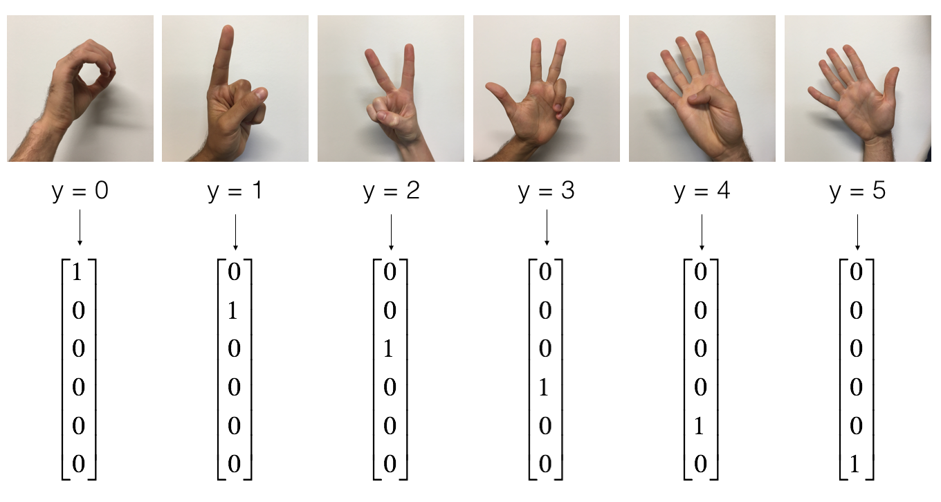
SIGNS 数据集是包含0到5的手势图。
1 | import math |
1 | # Loading the data (signs) |
1 | # Example of a picture |
y = 1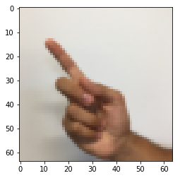
png
在前面的文章中,介绍了如何用全连接层对这个数据进行分类,本文将介绍使用CNN实现这个功能。
1 | X_train = X_train_orig/255. |
number of training examples = 1080
number of test examples = 120
X_train shape: (1080, 64, 64, 3)
Y_train shape: (1080, 6)
X_test shape: (120, 64, 64, 3)
Y_test shape: (120, 6)
建立模型
实现的模型CONV2D -> RELU -> MAXPOOL -> CONV2D -> RELU -> MAXPOOL -> FLATTEN -> FULLYCONNECTED。
建立占位符
Tensorflow要求先对输入数据建立占位符,然后塞入模型运行会话。
1 | # GRADED FUNCTION: create_placeholders |
1 | X, Y = create_placeholders(64, 64, 3, 6) |
X = Tensor("Placeholder:0", shape=(?, 64, 64, 3), dtype=float32)
Y = Tensor("Placeholder_1:0", shape=(?, 6), dtype=float32)
参数初始化
只需要对\(W1\)和\(W2\)进行初始化,全连接层和偏置量都不需要自己考虑,Tensorflow自动完成。
1 | # GRADED FUNCTION: initialize_parameters |
1 | tf.reset_default_graph() |
W1 = [ 0.00131723  0.14176141 -0.04434952  0.09197326  0.14984085 -0.03514394
 -0.06847463  0.05245192]
W2 = [-0.08566415  0.17750949  0.11974221  0.16773748 -0.0830943  -0.08058
 -0.00577033 -0.14643836  0.24162132 -0.05857408 -0.19055021  0.1345228
 -0.22779644 -0.1601823  -0.16117483 -0.10286498]
正传
tf.nn.conv2d(X,W1, strides = [1,s,s,1], padding = 'SAME'): 输入 \(X\) 和一组滤波器 \(W1\), 该函数对输入X应用褶积滤波器 \(W1\). 第3个输入 ([1,f,f,1]) 表示 在输入的每个维度上的步长 (m, n_H_prev, n_W_prev, n_C_prev). 参考详细文档 这里
tf.nn.max_pool(A, ksize = [1,f,f,1], strides = [1,s,s,1], padding = 'SAME'): 给定 A, 该函数应用窗口大小为 (f, f) 步长为(s, s) 实施最大池化. 参考详细文档 这里
tf.nn.relu(Z1): 对Z1 应用ReLU激活函数(点点运算,可以是任意维度的输入). 参考详细文档 这里.
tf.contrib.layers.flatten(P): 给定输入 P, 该函数在保留batch大小的情况下,将每个样本压扁为1D 向量. 生成压扁后的张量维度为 [batch_size, k]. 参考详细文档 这里.
tf.contrib.layers.fully_connected(F, num_outputs): 给定压扁后的张量 F, 返回全连接层的输出. 参考纤细文档 这里.
1 | # GRADED FUNCTION: forward_propagation |
1 | tf.reset_default_graph() |
Z3 = [[-0.44670227 -1.57208765 -1.53049231 -2.31013036 -1.29104376  0.46852064]
 [-0.17601591 -1.57972014 -1.4737016  -2.61672091 -1.00810647  0.5747785 ]]
计算代价函数
- tf.nn.softmax_cross_entropy_with_logits(logits = Z3, labels = Y): 计算softmax交叉熵损失函数. 该函数计算softmax 激活函数以及损失函数. 参考详细文档 这里.
- tf.reduce_mean: 计算一个张量所有维度上元素的平均值. 该函数计算所有样本损失之和,得到最终的代价. 参考详细文档 这里.
1 | # GRADED FUNCTION: compute_cost |
1 | tf.reset_default_graph() |
cost = 2.91034生成模型
将上面所有部分组合建立CNN模型,其中random_mini_batches()已经实现了选取mini-batch方法。
模型包括:
- 建立占位符
- 初始化参数
- 正传
- 计算代价函数
- 建立优化器
最终建立一个会话,执行for循环进行迭代,获取mini-batch,对每个mini-batch优化代价函数。参数初始化的详细信息请参考这里
1 | # GRADED FUNCTION: model |
1 | _, _, parameters = model(X_train, Y_train, X_test, Y_test) |
Cost after epoch 0: 1.917929
Cost after epoch 5: 1.506757
Cost after epoch 10: 0.955359
Cost after epoch 15: 0.845802
Cost after epoch 20: 0.701174
Cost after epoch 25: 0.571977
Cost after epoch 30: 0.518435
Cost after epoch 35: 0.495806
Cost after epoch 40: 0.429827
Cost after epoch 45: 0.407291
Cost after epoch 50: 0.366394
Cost after epoch 55: 0.376922
Cost after epoch 60: 0.299491
Cost after epoch 65: 0.338870
Cost after epoch 70: 0.316400
Cost after epoch 75: 0.310413
Cost after epoch 80: 0.249549
Cost after epoch 85: 0.243457
Cost after epoch 90: 0.200031
Cost after epoch 95: 0.175452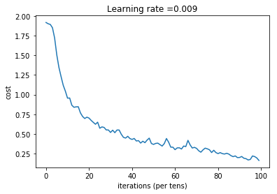
png
Tensor("Mean_1:0", shape=(), dtype=float32)
Train Accuracy: 0.940741
Test Accuracy: 0.783333
结论
使用Tensorflow实现CNN十分便捷,而且不需要自己编写反传和模型更新模块
参考资料
- 吴恩达,coursera深度学习课程