Keras搭建卷积神经网络

Keras是一种比Tensorflow更加高层次的深度学习编程框架，可以快速的构建深度神经网络，测试学习模型性能。本文介绍如何使用Keras搭建一个简单的卷积神经网络。

数据加载

import numpy as np
from keras import layers
from keras.layers import Input, Dense, Activation, ZeroPadding2D, BatchNormalization, Flatten, Conv2D
from keras.layers import AveragePooling2D, MaxPooling2D, Dropout, GlobalMaxPooling2D, GlobalAveragePooling2D
from keras.models import Model
from keras.preprocessing import image
from keras.utils import layer_utils
from keras.utils.data_utils import get_file
from keras.applications.imagenet_utils import preprocess_input
#import pydot
from IPython.display import SVG
from keras.utils.vis_utils import model_to_dot
from keras.utils import plot_model
from kt_utils import *

import keras.backend as K
K.set_image_data_format('channels_last')
import matplotlib.pyplot as plt
from matplotlib.pyplot import imshow

%matplotlib inline

X_train_orig, Y_train_orig, X_test_orig, Y_test_orig, classes = load_dataset()

# Normalize image vectors
X_train = X_train_orig/255.
X_test = X_test_orig/255.

# Reshape
Y_train = Y_train_orig.T
Y_test = Y_test_orig.T

print ("number of training examples = " + str(X_train.shape[0]))
print ("number of test examples = " + str(X_test.shape[0]))
print ("X_train shape: " + str(X_train.shape))
print ("Y_train shape: " + str(Y_train.shape))
print ("X_test shape: " + str(X_test.shape))
print ("Y_test shape: " + str(Y_test.shape))

number of training examples = 600
number of test examples = 150
X_train shape: (600, 64, 64, 3)
Y_train shape: (600, 1)
X_test shape: (150, 64, 64, 3)
Y_test shape: (150, 1)

"快乐" 数据集的详细信息:

图像的大小 (64,64,3)
训练集: 600幅图
测试集: 150幅图

在Keras中建立模型

一个建立学习模型的实例：

def model(input_shape):
    # Define the input placeholder as a tensor with shape input_shape. Think of this as your input image!
    X_input = Input(input_shape)

    # Zero-Padding: pads the border of X_input with zeroes
    X = ZeroPadding2D((3, 3))(X_input)

    # CONV -> BN -> RELU Block applied to X
    X = Conv2D(32, (7, 7), strides = (1, 1), name = 'conv0')(X)
    X = BatchNormalization(axis = 3, name = 'bn0')(X)
    X = Activation('relu')(X)

    # MAXPOOL
    X = MaxPooling2D((2, 2), name='max_pool')(X)

    # FLATTEN X (means convert it to a vector) + FULLYCONNECTED
    X = Flatten()(X)
    X = Dense(1, activation='sigmoid', name='fc')(X)

    # Create model. This creates your Keras model instance, you'll use this instance to train/test the model.
    model = Model(inputs = X_input, outputs = X, name='HappyModel')
    
    return model

从上面可以看出，和用numpy、tensorflwo不同，Keras每次都将计算结果覆盖到X输出，只有一个例外，就是X_input，这是因为后面还需要使用这个变量。

# GRADED FUNCTION: HappyModel

def HappyModel(input_shape):
    """
    Implementation of the HappyModel.
    
    Arguments:
    input_shape -- shape of the images of the dataset

    Returns:
    model -- a Model() instance in Keras
    """
    
    ### START CODE HERE ###
    # Feel free to use the suggested outline in the text above to get started, and run through the whole
    # exercise (including the later portions of this notebook) once. The come back also try out other
    # network architectures as well.
    # Define the input placeholder as a tensor with shape input_shape. Think of this as your input image!
    X_input = Input(input_shape)

    # Zero-Padding: pads the border of X_input with zeroes
    X = ZeroPadding2D((3, 3))(X_input)

    # CONV -> BN -> RELU Block applied to X
    X = Conv2D(32, (7, 7), strides = (1, 1), name = 'conv0')(X)
    X = BatchNormalization(axis = 3, name = 'bn0')(X)
    X = Activation('relu')(X)

    # MAXPOOL
    X = MaxPooling2D((2, 2), name='max_pool')(X)

    # FLATTEN X (means convert it to a vector) + FULLYCONNECTED
    X = Flatten()(X)
    X = Dense(1, activation='sigmoid', name='fc')(X)

    # Create model. This creates your Keras model instance, you'll use this instance to train/test the model.
    model = Model(inputs = X_input, outputs = X, name='HappyModel')

    return model
    
    
    
    ### END CODE HERE ###

在Keras建立学习模型的步骤包括：

利用上面的函数建立模型
调用model.compile(optimizer = "...", loss = "...", metrics = ["accuracy"])编译这个模型
调用model.fit(x = ..., y = ..., epochs = ..., batch_size = ...)训练模型
调用model.evaluate(x = ..., y = ...)使用测试数据测试模型

更多关于上面步骤的信息，请参考Keras文档.

1
2
3

### START CODE HERE ### (1 line)
happyModel = HappyModel(X_train.shape[1:])
### END CODE HERE ###

1
2
3

### START CODE HERE ### (1 line)
happyModel.compile(optimizer = 'adam', loss = 'binary_crossentropy', metrics= ['accuracy'])
### END CODE HERE ###

1
2
3

### START CODE HERE ### (1 line)
happyModel.fit(X_train, Y_train, epochs = 50, batch_size = 50)
### END CODE HERE ###

Epoch 1/50
600/600 [==============================] - 8s - loss: 2.9738 - acc: 0.5350     
Epoch 2/50
600/600 [==============================] - 8s - loss: 0.8352 - acc: 0.7033     
Epoch 3/50
600/600 [==============================] - 8s - loss: 0.3475 - acc: 0.8583     
Epoch 4/50
600/600 [==============================] - 8s - loss: 0.2112 - acc: 0.9117     
Epoch 5/50
600/600 [==============================] - 8s - loss: 0.1399 - acc: 0.9550     
Epoch 6/50
600/600 [==============================] - 8s - loss: 0.1190 - acc: 0.9633     
Epoch 7/50
600/600 [==============================] - 9s - loss: 0.1068 - acc: 0.9633     
Epoch 8/50
600/600 [==============================] - 8s - loss: 0.0944 - acc: 0.9717     
Epoch 9/50
600/600 [==============================] - 8s - loss: 0.0867 - acc: 0.9750     
Epoch 10/50
600/600 [==============================] - 8s - loss: 0.0792 - acc: 0.9850     
Epoch 11/50
600/600 [==============================] - 8s - loss: 0.0695 - acc: 0.9833     
Epoch 12/50
600/600 [==============================] - 8s - loss: 0.0628 - acc: 0.9833     
Epoch 13/50
600/600 [==============================] - 8s - loss: 0.0604 - acc: 0.9850     
Epoch 14/50
600/600 [==============================] - 8s - loss: 0.0563 - acc: 0.9850     
Epoch 15/50
600/600 [==============================] - 8s - loss: 0.0610 - acc: 0.9867     
Epoch 16/50
600/600 [==============================] - 8s - loss: 0.0491 - acc: 0.9883     
Epoch 17/50
600/600 [==============================] - 8s - loss: 0.0558 - acc: 0.9900     
Epoch 18/50
600/600 [==============================] - 8s - loss: 0.0476 - acc: 0.9883     
Epoch 19/50
600/600 [==============================] - 8s - loss: 0.0593 - acc: 0.9817     
Epoch 20/50
600/600 [==============================] - 8s - loss: 0.0506 - acc: 0.9867     
Epoch 21/50
600/600 [==============================] - 8s - loss: 0.0402 - acc: 0.9950     
Epoch 22/50
600/600 [==============================] - 8s - loss: 0.0431 - acc: 0.9883     
Epoch 23/50
600/600 [==============================] - 8s - loss: 0.0462 - acc: 0.9800     
Epoch 24/50
600/600 [==============================] - 8s - loss: 0.0648 - acc: 0.9817     
Epoch 25/50
600/600 [==============================] - 8s - loss: 0.0443 - acc: 0.9883     
Epoch 26/50
600/600 [==============================] - 8s - loss: 0.0360 - acc: 0.9883     
Epoch 27/50
600/600 [==============================] - 8s - loss: 0.0404 - acc: 0.9900     
Epoch 28/50
600/600 [==============================] - 8s - loss: 0.0371 - acc: 0.9917     
Epoch 29/50
600/600 [==============================] - 8s - loss: 0.0320 - acc: 0.9933     
Epoch 30/50
600/600 [==============================] - 8s - loss: 0.0207 - acc: 0.9950     
Epoch 31/50
600/600 [==============================] - 8s - loss: 0.0184 - acc: 0.9933     
Epoch 32/50
600/600 [==============================] - 8s - loss: 0.0159 - acc: 0.9983     
Epoch 33/50
600/600 [==============================] - 8s - loss: 0.0187 - acc: 0.9950     
Epoch 34/50
600/600 [==============================] - 8s - loss: 0.0225 - acc: 0.9917     
Epoch 35/50
600/600 [==============================] - 8s - loss: 0.0241 - acc: 0.9917     
Epoch 36/50
600/600 [==============================] - 8s - loss: 0.0241 - acc: 0.9883     
Epoch 37/50
600/600 [==============================] - 8s - loss: 0.0226 - acc: 0.9950     
Epoch 38/50
600/600 [==============================] - 8s - loss: 0.0173 - acc: 0.9933     
Epoch 39/50
600/600 [==============================] - 8s - loss: 0.0144 - acc: 0.9983     
Epoch 40/50
600/600 [==============================] - 8s - loss: 0.0114 - acc: 0.9983     
Epoch 41/50
600/600 [==============================] - 8s - loss: 0.0114 - acc: 0.9967     
Epoch 42/50
600/600 [==============================] - 8s - loss: 0.0087 - acc: 0.9983     
Epoch 43/50
600/600 [==============================] - 8s - loss: 0.0093 - acc: 0.9983     
Epoch 44/50
600/600 [==============================] - 8s - loss: 0.0153 - acc: 0.9983     
Epoch 45/50
600/600 [==============================] - 8s - loss: 0.0185 - acc: 0.9933     
Epoch 46/50
600/600 [==============================] - 8s - loss: 0.0259 - acc: 0.9917     
Epoch 47/50
600/600 [==============================] - 8s - loss: 0.0195 - acc: 0.9933     
Epoch 48/50
600/600 [==============================] - 8s - loss: 0.0170 - acc: 0.9950     
Epoch 49/50
600/600 [==============================] - 8s - loss: 0.0125 - acc: 0.9983     
Epoch 50/50
600/600 [==============================] - 8s - loss: 0.0284 - acc: 0.9933     





<keras.callbacks.History at 0x7fc206f5c198>

一些提升学习模型性能的策略：

使用一系列下面的模块CONV->BATCHNORM->RELU:

1
2
3

X = Conv2D(32, (3, 3), strides = (1, 1), name = 'conv0')(X)
X = BatchNormalization(axis = 3, name = 'bn0')(X)
X = Activation('relu')(X)

直到高、宽很小，深度很大（比如约等于32），这时表明你已经把有用的信息都编码到一个很多通道的数据体里，然后再压扁这个数据体，最后使用全连接层。
2. 在这些模块后使用MAXPOOL，降低高、宽的大小
3. 改变优化器，Adam一般都工作很好
4. 如果模型有内存问题，那么降低batch的大小
5. 执行更多的迭代次数，知道训练精度几乎不再提升

测试用户数据

### START CODE HERE ###
img_path = 'images/my_image.jpg'
### END CODE HERE ###
img = image.load_img(img_path, target_size=(64, 64))
imshow(img)

x = image.img_to_array(img)
x = np.expand_dims(x, axis=0)
x = preprocess_input(x)

print(happyModel.predict(x))

[[ 0.]]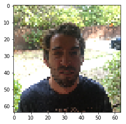

png

Keras其他一些有用的工具

model.summary(): 以表格形式打印每一层的详细信息以及输入输出信息
plot_model(): 画出模型

1	happyModel.summary()

_________________________________________________________________
Layer (type)                 Output Shape              Param #   
=================================================================
input_1 (InputLayer)         (None, 64, 64, 3)         0         
_________________________________________________________________
zero_padding2d_1 (ZeroPaddin (None, 70, 70, 3)         0         
_________________________________________________________________
conv0 (Conv2D)               (None, 64, 64, 32)        4736      
_________________________________________________________________
bn0 (BatchNormalization)     (None, 64, 64, 32)        128       
_________________________________________________________________
activation_1 (Activation)    (None, 64, 64, 32)        0         
_________________________________________________________________
max_pool (MaxPooling2D)      (None, 32, 32, 32)        0         
_________________________________________________________________
flatten_1 (Flatten)          (None, 32768)             0         
_________________________________________________________________
fc (Dense)                   (None, 1)                 32769     
=================================================================
Total params: 37,633
Trainable params: 37,569
Non-trainable params: 64
_________________________________________________________________

结论

Keras是一种十分方便的深度学习框架，非常适合快速上手
Keras的使用分为4步：建立模型->编译->训练->评估

参考资料

吴恩达，coursera深度学习课程