剩余网络（ResNets）

本文将介绍如何构建一种非常深的卷积神经网络，该网络称为剩余网络（ResNets）。理论上讲，非常深的网络可以刻画非常复杂的函数，但是实际上受梯度消失的影响，训练速度很慢，难以训练。本文介绍ResNets这种十分经典的深度卷积神经网络架构，并通过Keras编程框架一步一步构建ResNets网络。

###### import numpy as np
from keras import layers
from keras.layers import Input, Add, Dense, Activation, ZeroPadding2D, BatchNormalization, Flatten, Conv2D, AveragePooling2D, MaxPooling2D, GlobalMaxPooling2D
from keras.models import Model, load_model
from keras.preprocessing import image
from keras.utils import layer_utils
from keras.utils.data_utils import get_file
from keras.applications.imagenet_utils import preprocess_input
#import pydot
from IPython.display import SVG
from keras.utils.vis_utils import model_to_dot
from keras.utils import plot_model
from resnets_utils import *
from keras.initializers import glorot_uniform
import scipy.misc
from matplotlib.pyplot import imshow
%matplotlib inline

import keras.backend as K
K.set_image_data_format('channels_last')
K.set_learning_phase(1)

极深神经网络存在的问题

极深神经网络的主要优点是可以刻画十分复杂的函数。它可以从不同的抽象层面学习数据的特征，从边缘（浅层）到非常复杂的特征（深层）。但是网络越深，并不一定有帮助。训练这种网络十分重要的一个障碍是梯度消失：极深的网络往往梯度下降很快，直到接近于0，导致梯度下降法收敛十分缓慢。具体地讲，在梯度下降过程中，当信号从最后一层反传到第一层，需要在每一步乘以加权矩阵，因此梯度极有可能指数级下降到0（或者极少情况下指数级上升直到爆炸）。

在训练过程中，很有可能观察到：在训练过程中，浅层的梯度很快降到0，导致浅层更新很慢。

图 1 : 梯度消失
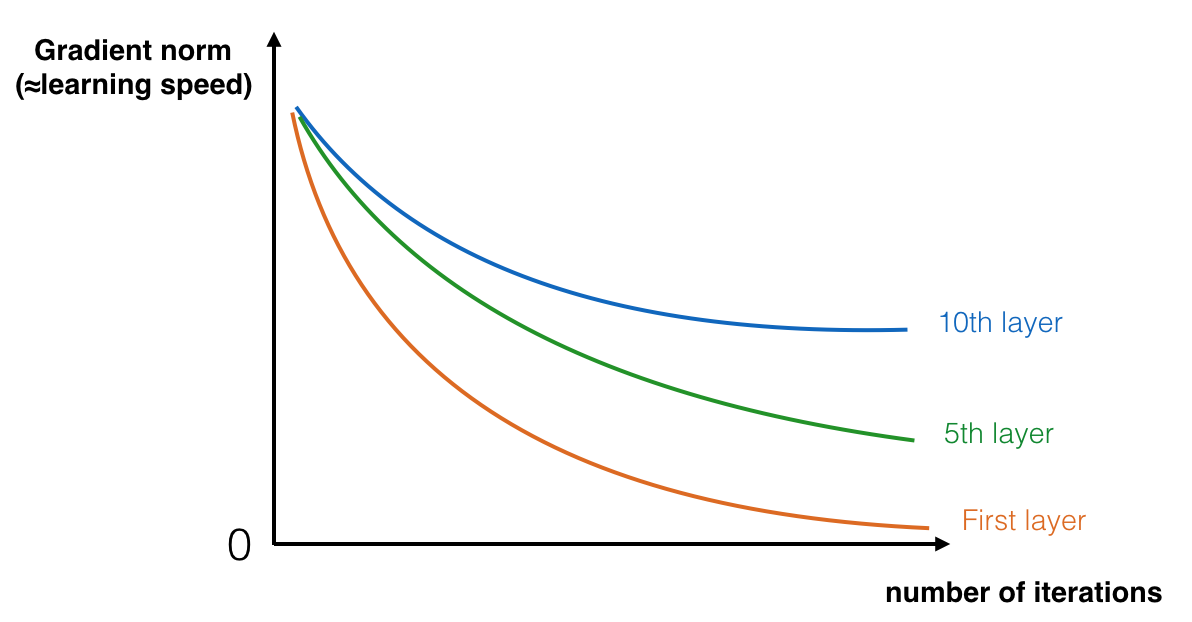
在网络的训练过程中，浅层的学习速度下降很快。

下面介绍如何使用剩余网络解决这个问题。

构建剩余网络

在ResNets中，shortcut或者skip连接允许梯度直接反传到浅层。

图 2 : ResNet模块skip-connection

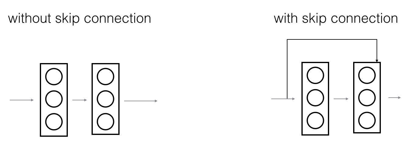
左图显示网络的主路径，右图在主路径上增加了一条捷径。将这些ResNet模块一级接一级，可以形成很深的网络。

带捷径的ResNet块使得每个模块很容易学到单位函数。也就意味着增加更多的ResNet模块不会增加太多影响训练性能的风险。（有证据表明：容易学到单位矩阵可以帮助解决梯度消失问题，也是ResNet性能强的原因。）

取决于输入/输入的维度是否相同，ResNet模块有两种主要的类型。

单位模块

单位模块是ResNets的标准模块，对应与输入激励 (比如\(a^{[l]}\)) 和(比如 \(a^{[l+2]}\))维度相同. 下面是ResNet中的单位模块:

图 3 : 单位模块. 跳跃连接层（“跳过”2 层）.

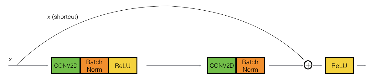
上面的路径是“捷径”，下面的路径是“主路径”。改图显式地画出了每一层中的CONV2D和ReLU。为了加快训练速度，同时也增加了BatchNorm。

下面的程序实际上实现了一种更加强大的单位模块，跳过3层。

Figure 4 : 单位模块. 跳跃连接层（ "跳过" 3 层）.

单位模块包括：

主路径的第一个部分：

第一个CONV2D滤波器\(F_1\) 大小为(1,1)，步长为 (1,1). padding 类型为 "valid" ，命名为 conv_name_base + '2a'. 0 为随机初始化的种子点.
第一个BatchNorm归一化深度方向. 命名为 bn_name_base + '2a'.
应用 ReLU 激活函数. 没有命名也没有超参参数.

主路径的第二部分: - 第二个CONV2D 滤波器 \(F_2\) 大小为\((f,f)\) ，步长为 (1,1). padding 类型为"same"，命名为 conv_name_base + '2b'. 0 为随机初始化的种子点.
- 第二个 BatchNorm 归一化深度方向. 命名为 bn_name_base + '2b'.
- 应用 ReLU 激活函数. 没有命名也没有超参.

主路径的第三部分: - 第三个 CONV2D 滤波器 \(F_3\) 大小为 (1,1)，步长为 (1,1). padding 类型为 "valid" ，命名为 conv_name_base + '2c'. 0 为随机初始化种子点.
- 第三个 BatchNorm 归一化深度方向. 命名为 bn_name_base + '2c'. 注意到这一部分没有激活函数.

最后一步: - 主路径输出和输入求和.
- 应用ReLU激活函数，没有命名也没有超参.

在Keras中： - 实现Conv2D，参考这里
- 实现BatchNorm，参考这里，（axis：整形，表示沿这个方向归一化，一般沿深度方向归一）
- 实现激活函数，使用Activation('relu')(X)
- 将捷径加入主路径输出，参考这里

# GRADED FUNCTION: identity_block

def identity_block(X, f, filters, stage, block):
    """
    Implementation of the identity block as defined in Figure 3
    
    Arguments:
    X -- input tensor of shape (m, n_H_prev, n_W_prev, n_C_prev)
    f -- integer, specifying the shape of the middle CONV's window for the main path
    filters -- python list of integers, defining the number of filters in the CONV layers of the main path
    stage -- integer, used to name the layers, depending on their position in the network
    block -- string/character, used to name the layers, depending on their position in the network
    
    Returns:
    X -- output of the identity block, tensor of shape (n_H, n_W, n_C)
    """
    
    # defining name basis
    conv_name_base = 'res' + str(stage) + block + '_branch'
    bn_name_base = 'bn' + str(stage) + block + '_branch'
    
    # Retrieve Filters
    F1, F2, F3 = filters
    
    # Save the input value. You'll need this later to add back to the main path. 
    X_shortcut = X
    
    # First component of main path
    X = Conv2D(filters = F1, kernel_size = (1, 1), strides = (1,1), padding = 'valid', name = conv_name_base + '2a', kernel_initializer = glorot_uniform(seed=0))(X)
    X = BatchNormalization(axis = 3, name = bn_name_base + '2a')(X)
    X = Activation('relu')(X)
    
    ### START CODE HERE ###
    
    # Second component of main path (≈3 lines)
    X = Conv2D(filters = F2, kernel_size = (f, f), strides = (1,1), padding = 'same', name = conv_name_base + '2b', kernel_initializer = glorot_uniform(seed=0))(X)
    X = BatchNormalization(axis = 3, name = bn_name_base + '2b')(X)
    X = Activation('relu')(X)

    # Third component of main path (≈2 lines)
    X = Conv2D(filters = F3, kernel_size = (1, 1), strides = (1,1), padding = 'valid', name = conv_name_base + '2c', kernel_initializer = glorot_uniform(seed=0))(X)
    X = BatchNormalization(axis = 3, name = bn_name_base + '2c')(X)

    # Final step: Add shortcut value to main path, and pass it through a RELU activation (≈2 lines)
    X = Add()([X, X_shortcut])
    X = Activation('relu')(X)
    
    ### END CODE HERE ###
    
    return X

tf.reset_default_graph()

with tf.Session() as test:
    np.random.seed(1)
    A_prev = tf.placeholder("float", [3, 4, 4, 6])
    X = np.random.randn(3, 4, 4, 6)
    A = identity_block(A_prev, f = 2, filters = [2, 4, 6], stage = 1, block = 'a')
    test.run(tf.global_variables_initializer())
    out = test.run([A], feed_dict={A_prev: X, K.learning_phase(): 0})
    print("out = " + str(out[0][1][1][0]))

out = [ 0.94822985  0.          1.16101444  2.747859    0.          1.36677003]

卷积模块

"卷积模块" 是ResNet中的另一种类型. 该模块用于输入输出维度不匹配的情况。和单位模块的区别在于捷径上是一个CONV2D层:

图 4 : 卷积模块

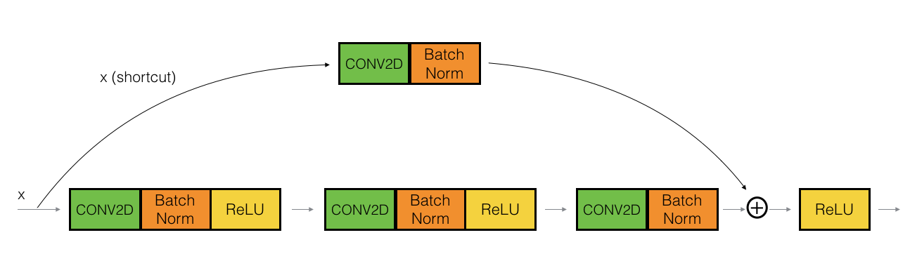
捷径上的 CONV2D 层用来对\(x\)重整为不同的维度, 使得捷径上的输出和主路径上的输出维度匹配，能够求和。捷径上的CONV2D 层不使用非线性激活函数. 其主要功能就是维度匹配.

卷积模块包括：

主路径的第一个部分：

第一个CONV2D滤波器\(F_1\) 大小为(1,1)，步长为 (1,1). padding 类型为 "valid" ，命名为 conv_name_base + '2a'. 0 为随机初始化的种子点.
第一个BatchNorm归一化深度方向. 命名为 bn_name_base + '2a'.
应用 ReLU 激活函数. 没有命名也没有超参参数.

捷径： - CONV2D 滤波器 \(F_3\) 大小为 (1,1) ，步长为 (s,s). padding 类型为 "valid" 命名为 conv_name_base + '1'.
- BatchNorm 归一化深度方向. 命名为 bn_name_base + '1'.

最后一步: - 主路径输出和捷径输入求和.
- 应用ReLU激活函数，没有命名也没有超参.

# GRADED FUNCTION: convolutional_block

def convolutional_block(X, f, filters, stage, block, s = 2):
    """
    Implementation of the convolutional block as defined in Figure 4
    
    Arguments:
    X -- input tensor of shape (m, n_H_prev, n_W_prev, n_C_prev)
    f -- integer, specifying the shape of the middle CONV's window for the main path
    filters -- python list of integers, defining the number of filters in the CONV layers of the main path
    stage -- integer, used to name the layers, depending on their position in the network
    block -- string/character, used to name the layers, depending on their position in the network
    s -- Integer, specifying the stride to be used
    
    Returns:
    X -- output of the convolutional block, tensor of shape (n_H, n_W, n_C)
    """
    
    # defining name basis
    conv_name_base = 'res' + str(stage) + block + '_branch'
    bn_name_base = 'bn' + str(stage) + block + '_branch'
    
    # Retrieve Filters
    F1, F2, F3 = filters
    
    # Save the input value
    X_shortcut = X


    ##### MAIN PATH #####
    # First component of main path 
    X = Conv2D(F1, (1, 1), strides = (s,s), name = conv_name_base + '2a', kernel_initializer = glorot_uniform(seed=0))(X)
    X = BatchNormalization(axis = 3, name = bn_name_base + '2a')(X)
    X = Activation('relu')(X)
    
    ### START CODE HERE ###

    # Second component of main path (≈3 lines)
    X = Conv2D(F2, (f, f), strides = (1,1), name = conv_name_base + '2b', padding = 'same', kernel_initializer = glorot_uniform(seed=0))(X)
    X = BatchNormalization(axis = 3, name = bn_name_base + '2b')(X)
    X = Activation('relu')(X)

    # Third component of main path (≈2 lines)
    X = Conv2D(F3, (1, 1), strides = (1,1), name = conv_name_base + '2c', padding = 'valid', kernel_initializer = glorot_uniform(seed=0))(X)
    X = BatchNormalization(axis = 3, name = bn_name_base + '2c')(X)

    ##### SHORTCUT PATH #### (≈2 lines)
    X_shortcut = Conv2D(F3, (1, 1), strides = (s,s), name = conv_name_base + '1', padding = 'valid', kernel_initializer = glorot_uniform(seed=0))(X_shortcut)
    X_shortcut = BatchNormalization(axis = 3, name = bn_name_base + '1')(X_shortcut)

    # Final step: Add shortcut value to main path, and pass it through a RELU activation (≈2 lines)
    X = Add()([X_shortcut,X])
    X = Activation('relu')(X)
    
    ### END CODE HERE ###
    
    return X

tf.reset_default_graph()

with tf.Session() as test:
    np.random.seed(1)
    A_prev = tf.placeholder("float", [3, 4, 4, 6])
    X = np.random.randn(3, 4, 4, 6)
    A = convolutional_block(A_prev, f = 2, filters = [2, 4, 6], stage = 1, block = 'a')
    test.run(tf.global_variables_initializer())
    out = test.run([A], feed_dict={A_prev: X, K.learning_phase(): 0})
    print("out = " + str(out[0][1][1][0]))

out = [ 0.09018463  1.23489773  0.46822017  0.0367176   0.          0.65516603]

构建第一个ResNet模型（50层）

现在已经实现了所有构建ResNet模型的组成部分. 图中"ID BLOCK" 代表 "单位模块"， "ID BLOCK x3" 表示链接 3 个单位模块.

图 5 : ResNet-50 模型

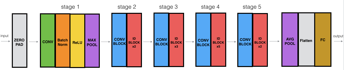
ResNet-50 模型细节: - Zero-padding pads the input with a pad of (3,3) - Stage 1: - The 2D Convolution has 64 filters of shape (7,7) and uses a stride of (2,2). Its name is "conv1". - BatchNorm is applied to the channels axis of the input. - MaxPooling uses a (3,3) window and a (2,2) stride. - Stage 2: - The convolutional block uses three set of filters of size [64,64,256], "f" is 3, "s" is 1 and the block is "a". - The 2 identity blocks use three set of filters of size [64,64,256], "f" is 3 and the blocks are "b" and "c". - Stage 3: - The convolutional block uses three set of filters of size [128,128,512], "f" is 3, "s" is 2 and the block is "a". - The 3 identity blocks use three set of filters of size [128,128,512], "f" is 3 and the blocks are "b", "c" and "d". - Stage 4: - The convolutional block uses three set of filters of size [256, 256, 1024], "f" is 3, "s" is 2 and the block is "a". - The 5 identity blocks use three set of filters of size [256, 256, 1024], "f" is 3 and the blocks are "b", "c", "d", "e" and "f". - Stage 5: - The convolutional block uses three set of filters of size [512, 512, 2048], "f" is 3, "s" is 2 and the block is "a". - The 2 identity blocks use three set of filters of size [512, 512, 2048], "f" is 3 and the blocks are "b" and "c". - The 2D Average Pooling uses a window of shape (2,2) and its name is "avg_pool". - The flatten doesn't have any hyperparameters or name. - The Fully Connected (Dense) layer reduces its input to the number of classes using a softmax activation. Its name should be 'fc' + str(classes).

函数说明: - Average pooling see reference

Here're some other functions we used in the code below: - Conv2D: See reference - BatchNorm: See reference (axis: Integer, the axis that should be normalized (typically the features axis)) - Zero padding: See reference - Max pooling: See reference - Fully conected layer: See reference - Addition: See reference

# GRADED FUNCTION: ResNet50

def ResNet50(input_shape = (64, 64, 3), classes = 6):
    """
    Implementation of the popular ResNet50 the following architecture:
    CONV2D -> BATCHNORM -> RELU -> MAXPOOL -> CONVBLOCK -> IDBLOCK*2 -> CONVBLOCK -> IDBLOCK*3
    -> CONVBLOCK -> IDBLOCK*5 -> CONVBLOCK -> IDBLOCK*2 -> AVGPOOL -> TOPLAYER

    Arguments:
    input_shape -- shape of the images of the dataset
    classes -- integer, number of classes

    Returns:
    model -- a Model() instance in Keras
    """
    
    # Define the input as a tensor with shape input_shape
    X_input = Input(input_shape)

    
    # Zero-Padding
    X = ZeroPadding2D((3, 3))(X_input)
    
    # Stage 1
    X = Conv2D(64, (7, 7), strides = (2, 2), name = 'conv1', kernel_initializer = glorot_uniform(seed=0))(X)
    X = BatchNormalization(axis = 3, name = 'bn_conv1')(X)
    X = Activation('relu')(X)
    X = MaxPooling2D((3, 3), strides=(2, 2))(X)

    # Stage 2
    X = convolutional_block(X, f = 3, filters = [64, 64, 256], stage = 2, block='a', s = 1)
    X = identity_block(X, 3, [64, 64, 256], stage=2, block='b')
    X = identity_block(X, 3, [64, 64, 256], stage=2, block='c')

    ### START CODE HERE ###

    # Stage 3 (≈4 lines)
    X = convolutional_block(X, f = 3, filters = [128, 128, 512], stage = 3, block='a', s = 2)
    X = identity_block(X, 3, [128, 128, 512], stage=3, block='b')
    X = identity_block(X, 3, [128, 128, 512], stage=3, block='c')
    X = identity_block(X, 3, [128, 128, 512], stage=3, block='d')

    # Stage 4 (≈6 lines)
    X = convolutional_block(X, f = 3, filters = [256, 256, 1024], stage = 4, block='a', s = 2)
    X = identity_block(X, 3, [256, 256, 1024], stage=4, block='b')
    X = identity_block(X, 3, [256, 256, 1024], stage=4, block='c')
    X = identity_block(X, 3, [256, 256, 1024], stage=4, block='d')
    X = identity_block(X, 3, [256, 256, 1024], stage=4, block='e')
    X = identity_block(X, 3, [256, 256, 1024], stage=4, block='f')

    # Stage 5 (≈3 lines)
    X = convolutional_block(X, f = 3, filters = [512, 512, 2048], stage = 5, block='a', s = 2)
    X = identity_block(X, 3, [512, 512, 2048], stage=5, block='b')
    X = identity_block(X, 3, [512, 512, 2048], stage=5, block='c')

    # AVGPOOL (≈1 line). Use "X = AveragePooling2D(...)(X)"
    X = AveragePooling2D(pool_size=(2,2))(X)
    
    ### END CODE HERE ###

    # output layer
    X = Flatten()(X)
    X = Dense(classes, activation='softmax', name='fc' + str(classes), kernel_initializer = glorot_uniform(seed=0))(X)
    
    
    # Create model
    model = Model(inputs = X_input, outputs = X, name='ResNet50')

    return model

建立模型计算图

1	model = ResNet50(input_shape = (64, 64, 3), classes = 6)

1	model.compile(optimizer='adam', loss='categorical_crossentropy', metrics=['accuracy'])

加载数据

X_train_orig, Y_train_orig, X_test_orig, Y_test_orig, classes = load_dataset()

# Normalize image vectors
X_train = X_train_orig/255.
X_test = X_test_orig/255.

# Convert training and test labels to one hot matrices
Y_train = convert_to_one_hot(Y_train_orig, 6).T
Y_test = convert_to_one_hot(Y_test_orig, 6).T

print ("number of training examples = " + str(X_train.shape[0]))
print ("number of test examples = " + str(X_test.shape[0]))
print ("X_train shape: " + str(X_train.shape))
print ("Y_train shape: " + str(Y_train.shape))
print ("X_test shape: " + str(X_test.shape))
print ("Y_test shape: " + str(Y_test.shape))

number of training examples = 1080
number of test examples = 120
X_train shape: (1080, 64, 64, 3)
Y_train shape: (1080, 6)
X_test shape: (120, 64, 64, 3)
Y_test shape: (120, 6)

训练模型

1	model.fit(X_train, Y_train, epochs = 2, batch_size = 32)

Epoch 1/2
1080/1080 [==============================] - 144s - loss: 3.0147 - acc: 0.2380   
Epoch 2/2
1080/1080 [==============================] - 143s - loss: 2.2702 - acc: 0.3167   





<keras.callbacks.History at 0x7ffae689afd0>

1
2
3

preds = model.evaluate(X_test, Y_test)
print ("Loss = " + str(preds[0]))
print ("Test Accuracy = " + str(preds[1]))

120/120 [==============================] - 5s     
Loss = 2.14528711637
Test Accuracy = 0.166666666667

增加更多的迭代次数，可以进一步改善性能。

结论

由于梯度消失，直接加深网络在实际中不会起作用。
跳跃连接层缓解了梯度消失问题，也使ResNet快容易学到单位函数；
ResNet模块有两种类型：单位模块和卷积模块。
通过连接更多的ResNet模块可以构建极深剩余网络。

参考资料

吴恩达，coursera深度学习课程
Kaiming He, Xiangyu Zhang, Shaoqing Ren, Jian Sun - Deep Residual Learning for Image Recognition (2015)
Francois Chollet's github repository: https://github.com/fchollet/deep-learning-models/blob/master/resnet50.py