本文将介绍一种功能强大的目标检测算法---YOLO算法。详细介绍YOLO算法的工作流程:输入图像经过CNN到编码数据体,再经阈值滤波和非最大值压制(NMS)去除多余的边框,最终得到目标检测结果及坐标。由于YOLO网络训练需要大量带标签数据以及强大计算量,本文使用已经训练好的网络,在Keras框架下,用一个汽车检测的例子展示这种算法的工作机制。
问题
在自动驾驶项目中,一个重要的部分是建立汽车检测系统。为了收集数据,在汽车前面安装摄像头,在汽车行驶过程中,每几秒拍摄道路前方的照片。
将这些照片收集起来并对每一辆汽车画上边框。加入你有80个类别需要YOLO算法识别出来,那么类别标签\(c\)可以表示成1到80的整数,或者一个80维的向量(one-hot编码,1的位置指示类别,剩余位置为0)。这两种标签方法都会用到,取决于在实际应用中哪一种更加方便。
YOLO算法
YOLO ("You Only Look Once") 是一种十分流行的算法,原因在于该算法精度很高,而且能够实时处理。“only look once"的意思是这个算法只需要在网络中一次正传就可以做预测。在经过non-max suppression,就可以输出识别的目标以及目标的边界。
模型的细节
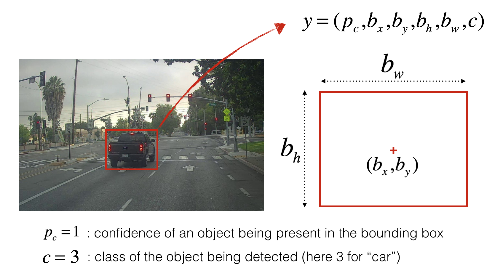
输入/输出信息: - 输入是一批大小为(m, 608, 608, 3)的图像 - 输出是一些列识别的类和带边界的窗口。每个边界用6个数字\((p_c, b_x, b_y, b_h, b_w, c)\)描述. 如果将类标签 \(c\) 展成80维的向量, 那么每个边框用85 数字描述.
本文用 5个 anchor 边框,所以YOLO的架构是: IMAGE (m, 608, 608, 3) -> DEEP CNN -> ENCODING (m, 19, 19, 5, 85).
YOLO算法的编码架构.
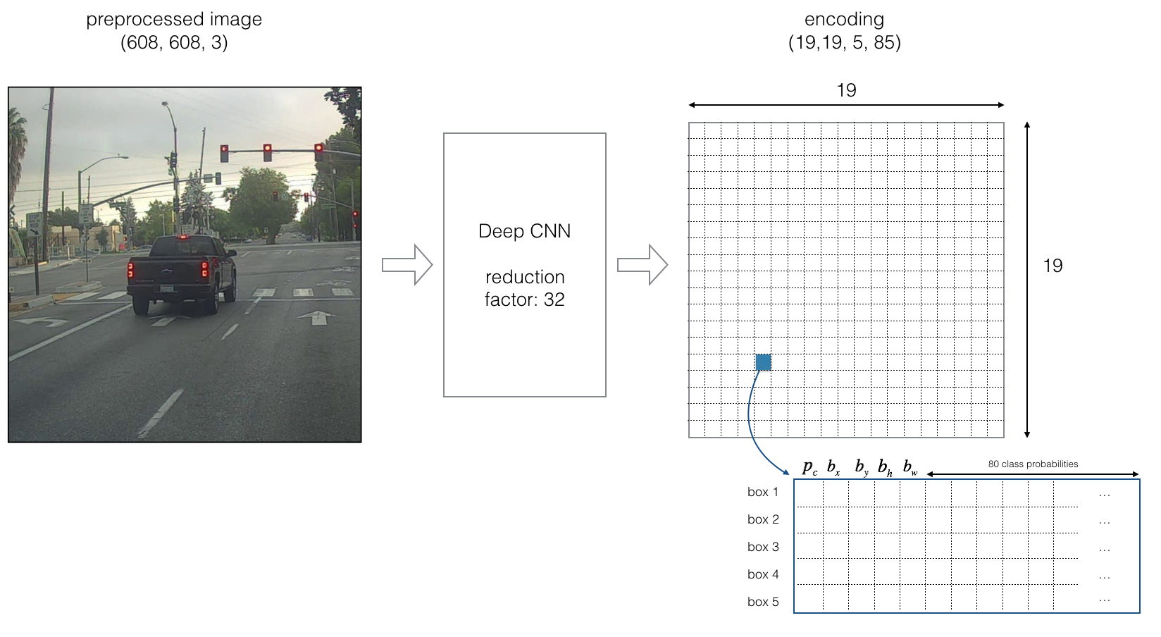
如果目标的中心店落入一个网格上,那么这个网格就负责探测这个目标。
由于我们使用了5个anchor边框,每个网格(总共19*19个)都编码了5种不同类型的边框,Anchor边框只由它的宽和高定义。
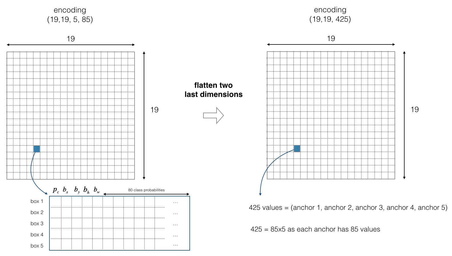
为简单期间, 编码输出 (19, 19, 5, 85) 最后两个维度做压扁处理,因此最后深度CNN的输出维度是19, 19, 425).
对于每一个网格,计算该网格包含某类目标的概率.
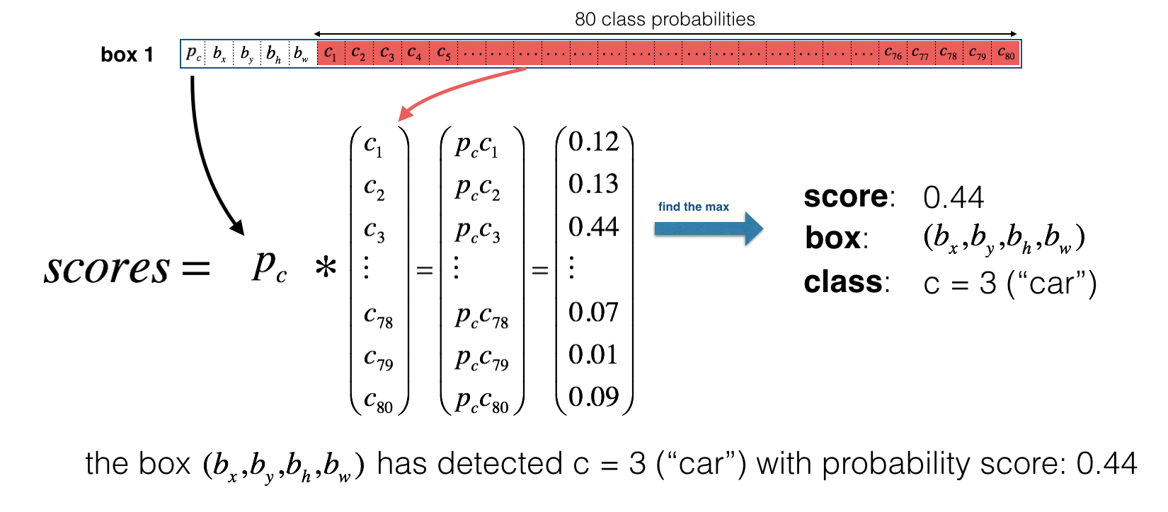
下面是一种可视化 YOLO算法预测结果的方法: - 对每个网格(共 19x19个) 寻找概率最大的类别 (包括5个anchor和80个类两个方向).
- 使用概率最大的类别,对网格进行颜色标定.
最后生成的图像为:
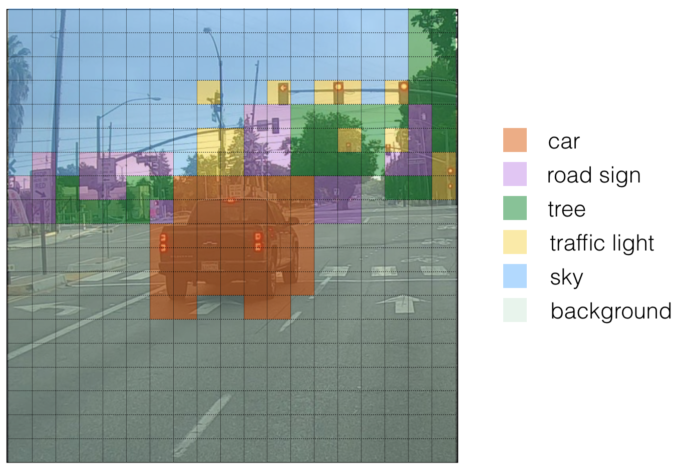
需要注意的是,这只是一种显示方式,并不是YOLO预测的核心部分。
另一种可视化的方式是将预测的边框都画出来. 如下图所示:
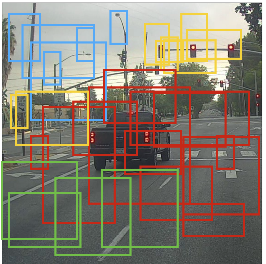
上面显示的是概率最大的边框,但是仍然很多。可以进一步通过non-max suppression去掉一些. 具体的步骤是:
- 去掉概率低的边框 (表示这个边框不是十分确信这是一个目标类)
- 当多个边框重叠并且表示同一个类时,只选择一个类.
根据分类概率滤掉一些边框
根据分类概率滤掉一些小于阈值的边框。
模型输出维度为19x19x5x85, 每个边框由 85 个数字描述. 将张量 (19,19,5,85) (或 (19,19,425)) 整成下面的变量:
- box_confidence: 维度为\((19 \times 19, 5, 1)\)的张量,表示每个网格(共19*19个)每种Anchor边框存在目标的置信概率 \(p_c\). - boxes: 维度为 \((19 \times 19, 5, 4)\)的张量,表示每个网格每种Anchor边框的形状 \((b_x, b_y, b_h, b_w)\). - box_class_probs: 维度为 \((19 \times 19, 5, 80)\)的张量,表示每个网格,每种Anchor边框,每种类别的概率 \((c_1, c_2, ... c_{80})\).
1 | import argparse |
Using TensorFlow backend.注意:由于将Keras的后台加载为K,意味着调用Keras函数需要K.function(...)
1 | # GRADED FUNCTION: yolo_filter_boxes |
1 | with tf.Session() as test_a: |
scores[2] = 10.7506
boxes[2] = [ 8.42653275  3.27136683 -0.53134358 -4.94137335]
classes[2] = 7
scores.shape = (?,)
boxes.shape = (?, 4)
classes.shape = (?,)注意:上面的?表示滤掉小概率事件后剩余的存在目标体的网格数量。
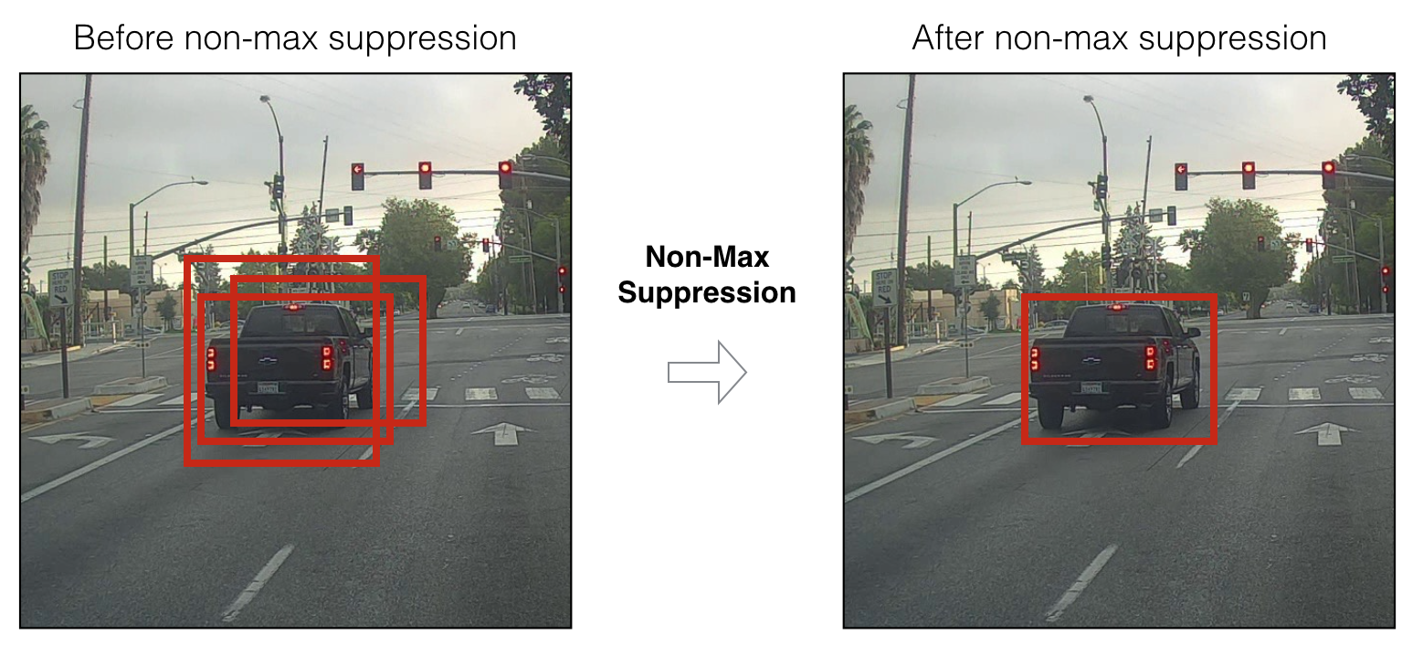
Non-max suppression
尽管根据分类概率用阈值滤掉了一些边框,但是仍然存在很多重叠的边框。第二种选择合理边框的方法是非最大值压制(NMS)
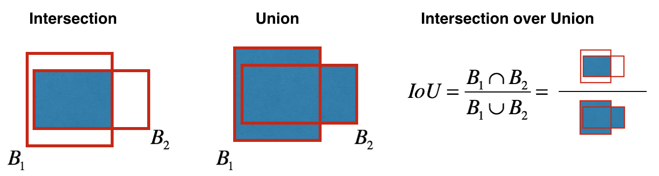
下面实现IOU函数: - 只在本文中,通过两个角点定义边框(左上角和右下角): (x1, y1, x2, y2) 而不是中心点和高/宽. - 计算一个矩形的面积:高(y2 - y1) × 宽 (x2 - x1) - 同样需要找到两个边框重叠的坐标 (xi1, yi1, xi2, yi2) : - xi1 = 两个边框x1 坐标的最大值
- yi1 = 两个边框y1 坐标的最大值
- xi2 = 两个边框x2 坐标的最小值 - yi2 = 两个边框y2 坐标的最小值
本例中 (0,0) 是图像的左上角, (1,0) 为图像的右上角, (1,1) 为图像的右下角.
1 | # GRADED FUNCTION: iou |
1 | box1 = (2, 1, 4, 3) |
iou = 0.142857142857实现NMS的主要步骤:
- 选择概率最高的边框
- 计算所有和这个边框重叠程度,移除重叠程度超过iou_threshold的边框
- 回到第一步迭代,直到没有比当前所选择边框概率更低的边框
上述过程将会移除所有和选定边框重叠率高的边框,仅仅剩下最优的边框。
1 | # GRADED FUNCTION: yolo_non_max_suppression |
1 | with tf.Session() as test_b: |
scores[2] = 6.9384
boxes[2] = [-5.299932    3.13798141  4.45036697  0.95942086]
classes[2] = -2.24527
scores.shape = (10,)
boxes.shape = (10, 4)
classes.shape = (10,)
包装前面的滤波器
深度CNN网络的输出维度为19x19x5x85,利用前面实现的函数(概率阈值和NMS)滤掉一些边框,即得到最终目标识别结果。 and filtering through all the boxes using the functions you've just implemented.
需要注意的是,边框有两种表示方式,一种是用角点,另一种是中点和高/宽。 YOLO经常要变换这两种方式:
1 | boxes = yolo_boxes_to_corners(box_xy, box_wh) |
上面将yolo边框坐标 (x,y,w,h) 转换成角点坐标 (x1, y1, x2, y2) 以作为函数 yolo_filter_boxes的输入 1
boxes = scale_boxes(boxes, image_shape)
YOLO网络实在608x608 的图像上训练得到的. 如果想用这个网络在不同大小的图像上测试,比如720x1280 的图像--上面的函数重尺度化边框大小,以画在 720x1280 的图像上.
1 | # GRADED FUNCTION: yolo_eval |
1 | with tf.Session() as test_b: |
scores[2] = 138.791
boxes[2] = [ 1292.32971191  -278.52166748  3876.98925781  -835.56494141]
classes[2] = 54
scores.shape = (10,)
boxes.shape = (10, 4)
classes.shape = (10,)
YOLO小结:
- 输入图像大小为(608, 608, 3)
- 输入图像进入CNN之后,输出维度为(19,19,5,85)
- 将最后两个维度压扁之后,维度为(19, 19, 425):
- 输入图像的每个网格对应 425 个数值.
- 425 = 5 x 85 表示每个网格包含5中不同的anchor边框.
- 85 = 5 + 80 其中5表示 \((p_c, b_x, b_y, b_h, b_w)\), \(p_c\)表示存在目标的概率、后面4个数值表示边框坐标,80表示要探测的目标类别数
- 只筛选出一小部分边框:
- 概率阈值筛选: 丢掉探测目标概率小于阈值的边框
- Non-max suppression: 计算重叠率IOU,避免选择重叠边框
- 概率阈值筛选: 丢掉探测目标概率小于阈值的边框
- 输出 YOLO算法的最终结果
测试已训练的YOLO模型
利用已经训练好的YOLO模型,对汽车数据集进行目标探测。和之前一样,首先建立会话,启动计算图
1 | sess = K.get_session() |
定义类别、anchor边框和图像大小
考虑探测80个类别,用5种anchor边框。所有80个类别和5种边框的信息都放在文件 "coco_classes.txt" 和 "yolo_anchors.txt"中. 用下面的命令加载这些数据。
汽车目标探测数据集的图像大小为720×1280,而YOLO模型处理的图像大小为608*608
1 | class_names = read_classes("model_data/coco_classes.txt") |
加载已训练好的YOLO模型
训练YOLO模型需要很长时间,也需要很大的标定数据集。本文加载一个已经用Keras训练好的 YOLO 模型——"yolo.h5". (权值来源于 YOLO 网站, 并被Allan Zelener转化成这种数据类型. 实际上,这些参数对应的是"YOLOv2" 模型, 但是这里还是简单称为"YOLO"模型.).
1 | yolo_model = load_model("model_data/yolo.h5") |
/home/seisinv/anaconda3/envs/tensorflow/lib/python3.5/site-packages/keras/models.py:258: UserWarning: No training configuration found in save file: the model was *not* compiled. Compile it manually.
  warnings.warn('No training configuration found in save file: '
1 | yolo_model.summary() |
____________________________________________________________________________________________________
Layer (type)                     Output Shape          Param #     Connected to
====================================================================================================
input_1 (InputLayer)             (None, 608, 608, 3)   0
____________________________________________________________________________________________________
conv2d_1 (Conv2D)                (None, 608, 608, 32)  864         input_1[0][0]
____________________________________________________________________________________________________
batch_normalization_1 (BatchNorm (None, 608, 608, 32)  128         conv2d_1[0][0]
____________________________________________________________________________________________________
leaky_re_lu_1 (LeakyReLU)        (None, 608, 608, 32)  0           batch_normalization_1[0][0]
____________________________________________________________________________________________________
max_pooling2d_1 (MaxPooling2D)   (None, 304, 304, 32)  0           leaky_re_lu_1[0][0]
____________________________________________________________________________________________________
conv2d_2 (Conv2D)                (None, 304, 304, 64)  18432       max_pooling2d_1[0][0]
____________________________________________________________________________________________________
batch_normalization_2 (BatchNorm (None, 304, 304, 64)  256         conv2d_2[0][0]
____________________________________________________________________________________________________
leaky_re_lu_2 (LeakyReLU)        (None, 304, 304, 64)  0           batch_normalization_2[0][0]
____________________________________________________________________________________________________
max_pooling2d_2 (MaxPooling2D)   (None, 152, 152, 64)  0           leaky_re_lu_2[0][0]
____________________________________________________________________________________________________
conv2d_3 (Conv2D)                (None, 152, 152, 128) 73728       max_pooling2d_2[0][0]
____________________________________________________________________________________________________
batch_normalization_3 (BatchNorm (None, 152, 152, 128) 512         conv2d_3[0][0]
____________________________________________________________________________________________________
leaky_re_lu_3 (LeakyReLU)        (None, 152, 152, 128) 0           batch_normalization_3[0][0]
____________________________________________________________________________________________________
conv2d_4 (Conv2D)                (None, 152, 152, 64)  8192        leaky_re_lu_3[0][0]
____________________________________________________________________________________________________
batch_normalization_4 (BatchNorm (None, 152, 152, 64)  256         conv2d_4[0][0]
____________________________________________________________________________________________________
leaky_re_lu_4 (LeakyReLU)        (None, 152, 152, 64)  0           batch_normalization_4[0][0]
____________________________________________________________________________________________________
conv2d_5 (Conv2D)                (None, 152, 152, 128) 73728       leaky_re_lu_4[0][0]
____________________________________________________________________________________________________
batch_normalization_5 (BatchNorm (None, 152, 152, 128) 512         conv2d_5[0][0]
____________________________________________________________________________________________________
leaky_re_lu_5 (LeakyReLU)        (None, 152, 152, 128) 0           batch_normalization_5[0][0]
____________________________________________________________________________________________________
max_pooling2d_3 (MaxPooling2D)   (None, 76, 76, 128)   0           leaky_re_lu_5[0][0]
____________________________________________________________________________________________________
conv2d_6 (Conv2D)                (None, 76, 76, 256)   294912      max_pooling2d_3[0][0]
____________________________________________________________________________________________________
batch_normalization_6 (BatchNorm (None, 76, 76, 256)   1024        conv2d_6[0][0]
____________________________________________________________________________________________________
leaky_re_lu_6 (LeakyReLU)        (None, 76, 76, 256)   0           batch_normalization_6[0][0]
____________________________________________________________________________________________________
conv2d_7 (Conv2D)                (None, 76, 76, 128)   32768       leaky_re_lu_6[0][0]
____________________________________________________________________________________________________
batch_normalization_7 (BatchNorm (None, 76, 76, 128)   512         conv2d_7[0][0]
____________________________________________________________________________________________________
leaky_re_lu_7 (LeakyReLU)        (None, 76, 76, 128)   0           batch_normalization_7[0][0]
____________________________________________________________________________________________________
conv2d_8 (Conv2D)                (None, 76, 76, 256)   294912      leaky_re_lu_7[0][0]
____________________________________________________________________________________________________
batch_normalization_8 (BatchNorm (None, 76, 76, 256)   1024        conv2d_8[0][0]
____________________________________________________________________________________________________
leaky_re_lu_8 (LeakyReLU)        (None, 76, 76, 256)   0           batch_normalization_8[0][0]
____________________________________________________________________________________________________
max_pooling2d_4 (MaxPooling2D)   (None, 38, 38, 256)   0           leaky_re_lu_8[0][0]
____________________________________________________________________________________________________
conv2d_9 (Conv2D)                (None, 38, 38, 512)   1179648     max_pooling2d_4[0][0]
____________________________________________________________________________________________________
batch_normalization_9 (BatchNorm (None, 38, 38, 512)   2048        conv2d_9[0][0]
____________________________________________________________________________________________________
leaky_re_lu_9 (LeakyReLU)        (None, 38, 38, 512)   0           batch_normalization_9[0][0]
____________________________________________________________________________________________________
conv2d_10 (Conv2D)               (None, 38, 38, 256)   131072      leaky_re_lu_9[0][0]
____________________________________________________________________________________________________
batch_normalization_10 (BatchNor (None, 38, 38, 256)   1024        conv2d_10[0][0]
____________________________________________________________________________________________________
leaky_re_lu_10 (LeakyReLU)       (None, 38, 38, 256)   0           batch_normalization_10[0][0]
____________________________________________________________________________________________________
conv2d_11 (Conv2D)               (None, 38, 38, 512)   1179648     leaky_re_lu_10[0][0]
____________________________________________________________________________________________________
batch_normalization_11 (BatchNor (None, 38, 38, 512)   2048        conv2d_11[0][0]
____________________________________________________________________________________________________
leaky_re_lu_11 (LeakyReLU)       (None, 38, 38, 512)   0           batch_normalization_11[0][0]
____________________________________________________________________________________________________
conv2d_12 (Conv2D)               (None, 38, 38, 256)   131072      leaky_re_lu_11[0][0]
____________________________________________________________________________________________________
batch_normalization_12 (BatchNor (None, 38, 38, 256)   1024        conv2d_12[0][0]
____________________________________________________________________________________________________
leaky_re_lu_12 (LeakyReLU)       (None, 38, 38, 256)   0           batch_normalization_12[0][0]
____________________________________________________________________________________________________
conv2d_13 (Conv2D)               (None, 38, 38, 512)   1179648     leaky_re_lu_12[0][0]
____________________________________________________________________________________________________
batch_normalization_13 (BatchNor (None, 38, 38, 512)   2048        conv2d_13[0][0]
____________________________________________________________________________________________________
leaky_re_lu_13 (LeakyReLU)       (None, 38, 38, 512)   0           batch_normalization_13[0][0]
____________________________________________________________________________________________________
max_pooling2d_5 (MaxPooling2D)   (None, 19, 19, 512)   0           leaky_re_lu_13[0][0]
____________________________________________________________________________________________________
conv2d_14 (Conv2D)               (None, 19, 19, 1024)  4718592     max_pooling2d_5[0][0]
____________________________________________________________________________________________________
batch_normalization_14 (BatchNor (None, 19, 19, 1024)  4096        conv2d_14[0][0]
____________________________________________________________________________________________________
leaky_re_lu_14 (LeakyReLU)       (None, 19, 19, 1024)  0           batch_normalization_14[0][0]
____________________________________________________________________________________________________
conv2d_15 (Conv2D)               (None, 19, 19, 512)   524288      leaky_re_lu_14[0][0]
____________________________________________________________________________________________________
batch_normalization_15 (BatchNor (None, 19, 19, 512)   2048        conv2d_15[0][0]
____________________________________________________________________________________________________
leaky_re_lu_15 (LeakyReLU)       (None, 19, 19, 512)   0           batch_normalization_15[0][0]
____________________________________________________________________________________________________
conv2d_16 (Conv2D)               (None, 19, 19, 1024)  4718592     leaky_re_lu_15[0][0]
____________________________________________________________________________________________________
batch_normalization_16 (BatchNor (None, 19, 19, 1024)  4096        conv2d_16[0][0]
____________________________________________________________________________________________________
leaky_re_lu_16 (LeakyReLU)       (None, 19, 19, 1024)  0           batch_normalization_16[0][0]
____________________________________________________________________________________________________
conv2d_17 (Conv2D)               (None, 19, 19, 512)   524288      leaky_re_lu_16[0][0]
____________________________________________________________________________________________________
batch_normalization_17 (BatchNor (None, 19, 19, 512)   2048        conv2d_17[0][0]
____________________________________________________________________________________________________
leaky_re_lu_17 (LeakyReLU)       (None, 19, 19, 512)   0           batch_normalization_17[0][0]
____________________________________________________________________________________________________
conv2d_18 (Conv2D)               (None, 19, 19, 1024)  4718592     leaky_re_lu_17[0][0]
____________________________________________________________________________________________________
batch_normalization_18 (BatchNor (None, 19, 19, 1024)  4096        conv2d_18[0][0]
____________________________________________________________________________________________________
leaky_re_lu_18 (LeakyReLU)       (None, 19, 19, 1024)  0           batch_normalization_18[0][0]
____________________________________________________________________________________________________
conv2d_19 (Conv2D)               (None, 19, 19, 1024)  9437184     leaky_re_lu_18[0][0]
____________________________________________________________________________________________________
batch_normalization_19 (BatchNor (None, 19, 19, 1024)  4096        conv2d_19[0][0]
____________________________________________________________________________________________________
conv2d_21 (Conv2D)               (None, 38, 38, 64)    32768       leaky_re_lu_13[0][0]
____________________________________________________________________________________________________
leaky_re_lu_19 (LeakyReLU)       (None, 19, 19, 1024)  0           batch_normalization_19[0][0]
____________________________________________________________________________________________________
batch_normalization_21 (BatchNor (None, 38, 38, 64)    256         conv2d_21[0][0]
____________________________________________________________________________________________________
conv2d_20 (Conv2D)               (None, 19, 19, 1024)  9437184     leaky_re_lu_19[0][0]
____________________________________________________________________________________________________
leaky_re_lu_21 (LeakyReLU)       (None, 38, 38, 64)    0           batch_normalization_21[0][0]
____________________________________________________________________________________________________
batch_normalization_20 (BatchNor (None, 19, 19, 1024)  4096        conv2d_20[0][0]
____________________________________________________________________________________________________
space_to_depth_x2 (Lambda)       (None, 19, 19, 256)   0           leaky_re_lu_21[0][0]
____________________________________________________________________________________________________
leaky_re_lu_20 (LeakyReLU)       (None, 19, 19, 1024)  0           batch_normalization_20[0][0]
____________________________________________________________________________________________________
concatenate_1 (Concatenate)      (None, 19, 19, 1280)  0           space_to_depth_x2[0][0]
                                                                   leaky_re_lu_20[0][0]
____________________________________________________________________________________________________
conv2d_22 (Conv2D)               (None, 19, 19, 1024)  11796480    concatenate_1[0][0]
____________________________________________________________________________________________________
batch_normalization_22 (BatchNor (None, 19, 19, 1024)  4096        conv2d_22[0][0]
____________________________________________________________________________________________________
leaky_re_lu_22 (LeakyReLU)       (None, 19, 19, 1024)  0           batch_normalization_22[0][0]
____________________________________________________________________________________________________
conv2d_23 (Conv2D)               (None, 19, 19, 425)   435625      leaky_re_lu_22[0][0]
====================================================================================================
Total params: 50,983,561
Trainable params: 50,962,889
Non-trainable params: 20,672
____________________________________________________________________________________________________
将模型的输出转化成有用的边框张量
yolo_model的输出维度为(m,19,19,5,85),需要进一步处理和转换。
1 | yolo_outputs = yolo_head(yolo_model.output, anchors, len(class_names)) |
边框滤波
yolo_outputs 得到的是 yolo_model输出的正确格式. 现在可以执行滤波,选择最优的边框。调用之前实现的 yolo_eval。
1 | scores, boxes, classes = yolo_eval(yolo_outputs, image_shape) |
在一张图像上执行计算图
建立计算图 (sess) 的流程为:
- yolo_model.input 输入
yolo_model. 该模型用来计算输出 yolo_model.output - yolo_model.output 经
yolo_head处理. 输出 yolo_outputs - yolo_outputs 进入滤波函数,
yolo_eval. 输出预测结果: scores, boxes, classes
使用的函数包括: 1
image, image_data = preprocess_image("images/" + image_file, model_image_size = (608, 608))
输出:
- image: 用于图像画边框的python (PIL) 表示.
- image_data: 图像的NUMPY表示. 作为 CNN的输入.
注意: 当模型使用 BatchNorm (比如YOLO模型), 需要在字典feed_dict中传递另一个占位符 {K.learning_phase(): 0}.
1 | def predict(sess, image_file): |
1 | out_scores, out_boxes, out_classes = predict(sess, "test.jpg") |
Found 7 boxes for test.jpg
car 0.60 (925, 285) (1045, 374)
car 0.66 (706, 279) (786, 350)
bus 0.67 (5, 266) (220, 407)
car 0.70 (947, 324) (1280, 705)
car 0.74 (159, 303) (346, 440)
car 0.80 (761, 282) (942, 412)
car 0.89 (367, 300) (745, 648)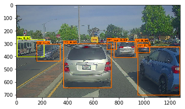
png
结论
- YOLO是当前既快、又准确的目标检测模型
- 输入图像经过CNN之后,输出\(19\times19\times5\times85\)维数据体
- 输出可看做是19*19网格上每个网格5中不同边框的信息
- 对所有边框实施非最大值压制,具体包括:
- 利用阈值过滤掉概率小的目标检测结果
- 计算IoU去掉覆盖率高的边框
- 由于从随机权值开始训练YOLO模型,需要很大的数据集和计算量,本文使用已经训练的模型。
参考资料
- 吴恩达,coursera深度学习课程
- Joseph Redmon, Santosh Divvala, Ross Girshick, Ali Farhadi - You Only Look Once: Unified, Real-Time Object Detection (2015)
- Joseph Redmon, Ali Farhadi - YOLO9000: Better, Faster, Stronger (2016)
- Allan Zelener - YAD2K: Yet Another Darknet 2 Keras
- The official YOLO website (https://pjreddie.com/darknet/yolo/)
Car detection dataset: 
The Drive.ai Sample Dataset (provided by drive.ai) is licensed under a Creative Commons Attribution 4.0 International License. We are especially grateful to Brody Huval, Chih Hu and Rahul Patel for collecting and providing this dataset.