风格转换

在深度学习中，大多数的应用都是优化神经网络参数。在风格转换中，将是优化图像的像素值。本文利用事先训练好的VGG模型提取图像特征，然后利用隐藏层的特征信息计算内容代价函数和风格代价函数，通过最小化这连个代价函数之和，优化合成图像的像素值，得到风格转换之后的新图像。

问题阐述

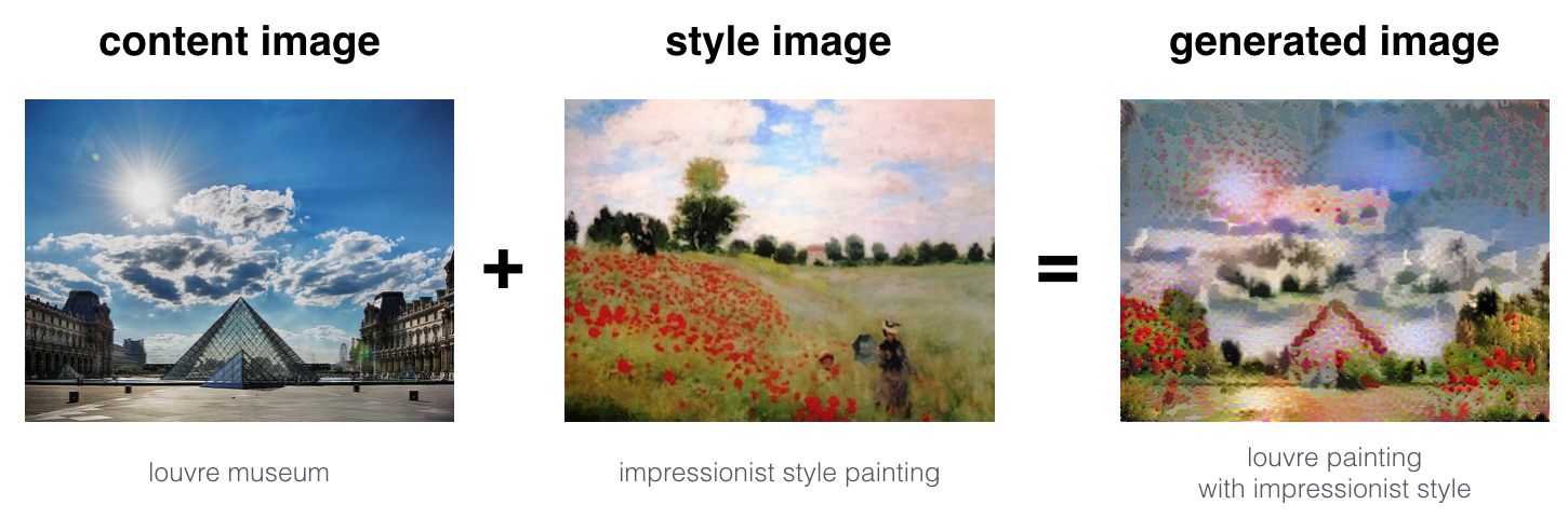
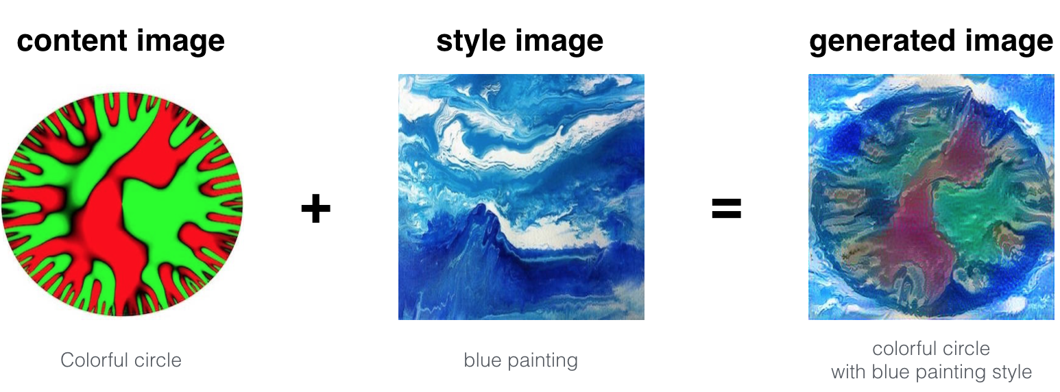
神经网络风格转换(Neural Style Transfer: NST)，是深度学习中十分有意思的一项技术。它将两张图像：一张为“内容"图像(C)，一张为"风格"图像(S)，产生"合成"图像(G)。合成图像既有图像C的内容，又有图像S的风格。

迁移学习

风格转换使用事先训练好的模型，在此基础上构建新模型。将一种任务训练的模型应用到另一种任务的想法，常称之为迁移学习

本文采用VGG网络，具体是VGG-19网络。该网络是通过ImageNet数据库训练出来的。

import os
import sys
import scipy.io
import scipy.misc
import matplotlib.pyplot as plt
from matplotlib.pyplot import imshow
from PIL import Image
from nst_utils import *
import numpy as np
import tensorflow as tf

%matplotlib inline

1 2	model = load_vgg_model("pretrained-model/imagenet-vgg-verydeep-19.mat") print(model)

{'conv5_2': <tf.Tensor 'Relu_13:0' shape=(1, 19, 25, 512) dtype=float32>, 'conv3_1': <tf.Tensor 'Relu_4:0' shape=(1, 75, 100, 256) dtype=float32>, 'conv3_2': <tf.Tensor 'Relu_5:0' shape=(1, 75, 100, 256) dtype=float32>, 'conv5_3': <tf.Tensor 'Relu_14:0' shape=(1, 19, 25, 512) dtype=float32>, 'avgpool1': <tf.Tensor 'AvgPool:0' shape=(1, 150, 200, 64) dtype=float32>, 'conv2_1': <tf.Tensor 'Relu_2:0' shape=(1, 150, 200, 128) dtype=float32>, 'conv1_1': <tf.Tensor 'Relu:0' shape=(1, 300, 400, 64) dtype=float32>, 'conv2_2': <tf.Tensor 'Relu_3:0' shape=(1, 150, 200, 128) dtype=float32>, 'conv5_1': <tf.Tensor 'Relu_12:0' shape=(1, 19, 25, 512) dtype=float32>, 'conv5_4': <tf.Tensor 'Relu_15:0' shape=(1, 19, 25, 512) dtype=float32>, 'avgpool5': <tf.Tensor 'AvgPool_4:0' shape=(1, 10, 13, 512) dtype=float32>, 'conv1_2': <tf.Tensor 'Relu_1:0' shape=(1, 300, 400, 64) dtype=float32>, 'avgpool3': <tf.Tensor 'AvgPool_2:0' shape=(1, 38, 50, 256) dtype=float32>, 'conv3_3': <tf.Tensor 'Relu_6:0' shape=(1, 75, 100, 256) dtype=float32>, 'conv4_1': <tf.Tensor 'Relu_8:0' shape=(1, 38, 50, 512) dtype=float32>, 'avgpool4': <tf.Tensor 'AvgPool_3:0' shape=(1, 19, 25, 512) dtype=float32>, 'conv4_3': <tf.Tensor 'Relu_10:0' shape=(1, 38, 50, 512) dtype=float32>, 'conv3_4': <tf.Tensor 'Relu_7:0' shape=(1, 75, 100, 256) dtype=float32>, 'avgpool2': <tf.Tensor 'AvgPool_1:0' shape=(1, 75, 100, 128) dtype=float32>, 'conv4_2': <tf.Tensor 'Relu_9:0' shape=(1, 38, 50, 512) dtype=float32>, 'input': <tf.Variable 'Variable:0' shape=(1, 300, 400, 3) dtype=float32_ref>, 'conv4_4': <tf.Tensor 'Relu_11:0' shape=(1, 38, 50, 512) dtype=float32>}

模型存储在一个python字典中，关键字为变量名，对应的值为包含这个变量数值的张量。使用这个网络时，将图像喂进这个模型带即可。

1	model["input"].assign(image)

如果想获得某一层的某些激励，比如层4_2，可以运行下面的对话：

1	sess.run(model["conv4_2"])

实现NST算法分为3步：

建立内容代价函数 $J_{content}(C,G)$
建立风格代价函数 $J_{style}(S,G)$
结合这两个代价函数 $J(G) = \alpha J_{content}(C,G) + \beta J_{style}(S,G)$.

计算内容代价函数

CNN浅层对应的是简单的特征，深层对应的是复制的特征。对于风格转换这一应用而言，最好选择不深也不浅的层。

假定C是事先训练好的VGG网络的输入，进行正传之后，假定 $a^{(C)}$ 是选定隐藏层激活函数输出，是维度为 $n_H \times n_W \times n_C$ 的张量. 对G重复以下过程: 以 G 作为输入进行正传. 令 \[a^{(G)}\] 为选定隐藏层的输出. 定义内容代价函数为:

\[J_{content}(C,G) = \frac{1}{4 \times n_H \times n_W \times n_C}\sum _{ \text{all entries}} (a^{(C)} - a^{(G)})^2\tag{1} \]

其中 $n_H, n_W$ 和 $n_C$ 为选定隐藏层的高、宽和深度。$a^{(C)}$ 和 $a^{(G)}$ 都是选定隐藏层的输出.

1 2	content_image = scipy.misc.imread("images/louvre.jpg") imshow(content_image)

<matplotlib.image.AxesImage at 0x7f26bd126f60>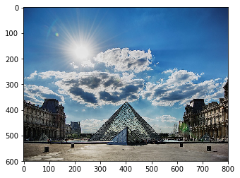

png

# GRADED FUNCTION: compute_content_cost

def compute_content_cost(a_C, a_G):
    """
    Computes the content cost
    
    Arguments:
    a_C -- tensor of dimension (1, n_H, n_W, n_C), hidden layer activations representing content of the image C 
    a_G -- tensor of dimension (1, n_H, n_W, n_C), hidden layer activations representing content of the image G
    
    Returns: 
    J_content -- scalar that you compute using equation 1 above.
    """
    
    ### START CODE HERE ###
    # Retrieve dimensions from a_G (≈1 line)
    m, n_H, n_W, n_C = a_G.get_shape().as_list()
    
    # Reshape a_C and a_G (≈2 lines)
    a_C_unrolled = tf.transpose(tf.reshape(a_C, [1,n_H*n_W,n_C]))
    a_G_unrolled = tf.transpose(tf.reshape(a_G, [1,n_H*n_W,n_C]))
    
    # compute the cost with tensorflow (≈1 line)
    J_content = (1/(4*n_H*n_W*n_C))*tf.reduce_sum(tf.square(tf.subtract(a_C_unrolled,a_G_unrolled)))
    ### END CODE HERE ###
    
    return J_content

tf.reset_default_graph()

with tf.Session() as test:
    tf.set_random_seed(1)
    a_C = tf.random_normal([1, 4, 4, 3], mean=1, stddev=4)
    a_G = tf.random_normal([1, 4, 4, 3], mean=1, stddev=4)
    J_content = compute_content_cost(a_C, a_G)
    print("J_content = " + str(J_content.eval()))

J_content = 6.76559

小结

内容代价函数取神经网络隐藏层的输出，并测量^{(C)}$ 和 $a^{(G)}$的差异
当最小内容化代价函数，会使得$G$和$C$内容相似

计算风格代价函数

1 2	style_image = scipy.misc.imread("images/monet_800600.jpg") imshow(style_image)

<matplotlib.image.AxesImage at 0x7f26bc0989e8>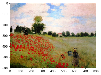

png

风格矩阵

风格矩阵也称为"Gram"矩阵。在线性袋鼠中，Gram 矩阵 G 是一系列向量集合 $(v_{1},\dots ,v_{n})$ 的点乘, 其元素 ${\displaystyle G_{ij} = v_{i}^T v_{j} = np.dot(v_{i}, v_{j}) }$. 换句话说， $G_{ij}$ 计算 $v_i$ 和$v_j$的相似度: 如果它们十分相似, 则输出大的点乘结果, 也就是 $G_{ij}$会比较大.

Note that there is an unfortunate collision in the variable names used here. We are following common terminology used in the literature, but $G$ is used to denote the Style matrix (or Gram matrix) as well as to denote the generated image $G$. We will try to make sure which $G$ we are referring to is always clear from the context.

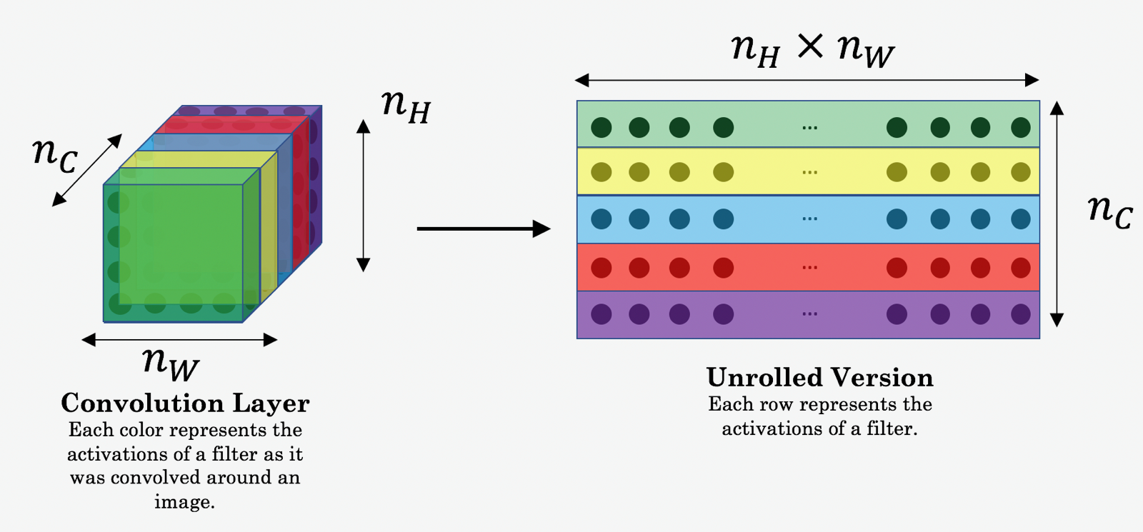
在风格转换中，Style 矩阵是计算 "展开" 之后矩阵和它的专制之间的乘积:

最终的矩阵维度为 $(n_C,n_C)$，其中 $n_C$ 是滤波器的而个数.$G_{ij}$表示滤波器$i$ 和滤波器$j$输出的相似度。

Gram 矩阵的对角线元素$G_{ii}$ 测量的是滤波器 $i$ 的激活程度. 例如，假定滤波器 $i$ 探测是图像的垂直纹理，那么$G_{ii}$测量的是整个图像中垂直纹理的普遍程度: 如果 $G_{ii}$ 很大, 表明这幅图像存在很多垂直纹理。

通过获取不同类型的特征的普遍程度 ($G_{ii}$)以及不同特征同时存在的程度($G_{ij}$), 风格矩阵 $G$ 定量测量了一幅图像的风格.

# GRADED FUNCTION: gram_matrix

def gram_matrix(A):
    """
    Argument:
    A -- matrix of shape (n_C, n_H*n_W)
    
    Returns:
    GA -- Gram matrix of A, of shape (n_C, n_C)
    """
    
    ### START CODE HERE ### (≈1 line)
    GA = tf.matmul(A,tf.transpose(A))
    ### END CODE HERE ###
    
    return GA

tf.reset_default_graph()

with tf.Session() as test:
    tf.set_random_seed(1)
    A = tf.random_normal([3, 2*1], mean=1, stddev=4)
    GA = gram_matrix(A)
    
    print("GA = " + str(GA.eval()))

GA = [[  6.42230511  -4.42912197  -2.09668207]
 [ -4.42912197  19.46583748  19.56387138]
 [ -2.09668207  19.56387138  20.6864624 ]]

风格代价函数

生成风格矩阵 (Gram 矩阵)之后,目标是减小 “风格”图像 S 和“合成”图像 G 之间Gram matrix之间的距离. 这里只使用一层的激励 $a^{[l]}$, 对应的风格代价函数为:

\[J_{style}^{[l]}(S,G) = \frac{1}{4 \times {n_C}^2 \times (n_H \times n_W)^2} \sum _{i=1}^{n_C}\sum_{j=1}^{n_C}(G^{(S)}_{ij} - G^{(G)}_{ij})^2\tag{2} \]

其中 $G^{(S)}$ and $G^{(G)}$ 分别是风格图像S和合成图像的Gram矩阵, 输入是来自与同一特定隐藏层的激励.

# GRADED FUNCTION: compute_layer_style_cost

def compute_layer_style_cost(a_S, a_G):
    """
    Arguments:
    a_S -- tensor of dimension (1, n_H, n_W, n_C), hidden layer activations representing style of the image S 
    a_G -- tensor of dimension (1, n_H, n_W, n_C), hidden layer activations representing style of the image G
    
    Returns: 
    J_style_layer -- tensor representing a scalar value, style cost defined above by equation (2)
    """
    
    ### START CODE HERE ###
    # Retrieve dimensions from a_G (≈1 line)
    m, n_H, n_W, n_C = a_G.get_shape().as_list()
    
    # Reshape the images to have them of shape (n_C, n_H*n_W) (≈2 lines)
    a_S = tf.reshape(a_S, [n_H*n_W, n_C])
    a_G = tf.reshape(a_G, [n_H*n_W, n_C])

    # Computing gram_matrices for both images S and G (≈2 lines)
    GS = gram_matrix(tf.transpose(a_S))
    GG = gram_matrix(tf.transpose(a_G))

    # Computing the loss (≈1 line)
    J_style_layer = (1/(4*(n_C**2)*((n_H*n_W)**2)))*tf.reduce_sum(tf.square(tf.subtract(GS,GG)))
    
    ### END CODE HERE ###
    
    return J_style_layer

tf.reset_default_graph()

with tf.Session() as test:
    tf.set_random_seed(1)
    a_S = tf.random_normal([1, 4, 4, 3], mean=1, stddev=4)
    a_G = tf.random_normal([1, 4, 4, 3], mean=1, stddev=4)
    J_style_layer = compute_layer_style_cost(a_S, a_G)
    
    print("J_style_layer = " + str(J_style_layer.eval()))

J_style_layer = 9.19028

风格权值

上面值考虑了一层的风格信息。实际上，可以考虑多层，并用合理的权值将它们合并成新的风格矩阵。例如下面的权值：

STYLE_LAYERS = [
    ('conv1_1', 0.2),
    ('conv2_1', 0.2),
    ('conv3_1', 0.2),
    ('conv4_1', 0.2),
    ('conv5_1', 0.2)]

风格代价函数可以通过下面的公式计算：

\[J_{style}(S,G) = \sum_{l} \lambda^{[l]} J^{[l]}_{style}(S,G)\]

其中$\lambda^{[l]}$ 值在变量 STYLE_LAYERS中给定。

前面已经实现了函数compute_style_cost(...). 多次调用这个函数，然后对结果利用STYLE_LAYERS中的权系数加权求和，则得到最终的风格代价函数.

def compute_style_cost(model, STYLE_LAYERS):
    """
    Computes the overall style cost from several chosen layers
    
    Arguments:
    model -- our tensorflow model
    STYLE_LAYERS -- A python list containing:
                        - the names of the layers we would like to extract style from
                        - a coefficient for each of them
    
    Returns: 
    J_style -- tensor representing a scalar value, style cost defined above by equation (2)
    """
    
    # initialize the overall style cost
    J_style = 0

    for layer_name, coeff in STYLE_LAYERS:

        # Select the output tensor of the currently selected layer
        out = model[layer_name]

        # Set a_S to be the hidden layer activation from the layer we have selected, by running the session on out
        a_S = sess.run(out)

        # Set a_G to be the hidden layer activation from same layer. Here, a_G references model[layer_name] 
        # and isn't evaluated yet. Later in the code, we'll assign the image G as the model input, so that
        # when we run the session, this will be the activations drawn from the appropriate layer, with G as input.
        a_G = out
        
        # Compute style_cost for the current layer
        J_style_layer = compute_layer_style_cost(a_S, a_G)

        # Add coeff * J_style_layer of this layer to overall style cost
        J_style += coeff * J_style_layer

    return J_style

小结

隐藏层的输出形成Gamma矩阵，可以用来定量化图像的风格。通过结合更多隐藏层的信息，可以更好的代表图像的风格。相对而言，内容信息往往只需要一个隐藏层的信息。
最小化风格代价函数，就可以使得图像G变得和图像S的风格类似

定义总的代价函数

最后结合内容代价函数和风格代价函数：

\[J(G) = \alpha J_{content}(C,G) + \beta J_{style}(S,G)\]

# GRADED FUNCTION: total_cost

def total_cost(J_content, J_style, alpha = 10, beta = 40):
    """
    Computes the total cost function
    
    Arguments:
    J_content -- content cost coded above
    J_style -- style cost coded above
    alpha -- hyperparameter weighting the importance of the content cost
    beta -- hyperparameter weighting the importance of the style cost
    
    Returns:
    J -- total cost as defined by the formula above.
    """
    
    ### START CODE HERE ### (≈1 line)
    J = alpha*J_content + beta*J_style
    ### END CODE HERE ###
    
    return J

tf.reset_default_graph()

with tf.Session() as test:
    np.random.seed(3)
    J_content = np.random.randn()    
    J_style = np.random.randn()
    J = total_cost(J_content, J_style)
    print("J = " + str(J))

J = 35.34667875478276

最优化问题求解

解决风格转换这个优化问题的流程：

建立交互会话
加载内容图像
加载风格图像
对合成图像随机初始化
加载VGG16模型
建立Tensorflow计算图：

输入内容图像到VGG16模型，计算内容代价函数
输入风格图像到VGG16模型，计算风格代价函数
计算总代价函数
定义最优化对象和学习率

初始化Tensoflow图，迭代多次，每次迭代更新合成图像

# Reset the graph
tf.reset_default_graph()

# Start interactive session
sess = tf.InteractiveSession()

1 2	content_image = scipy.misc.imread("images/louvre_small.jpg") content_image = reshape_and_normalize_image(content_image)

1 2	style_image = scipy.misc.imread("images/monet.jpg") style_image = reshape_and_normalize_image(style_image)

尽管是随机初始化合成图像，但是仍然让其和内容图像轻微相关，这样可以加快收敛速度。

1 2	generated_image = generate_noise_image(content_image) imshow(generated_image[0])

<matplotlib.image.AxesImage at 0x7f26b47a0ef0>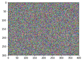

png

model = load_vgg_model("pretrained-model/imagenet-vgg-verydeep-19.mat")# Assign the content image to be the input of the VGG model.  
sess.run(model['input'].assign(content_image))

# Select the output tensor of layer conv4_2
out = model['conv4_2']

# Set a_C to be the hidden layer activation from the layer we have selected
a_C = sess.run(out)

# Set a_G to be the hidden layer activation from same layer. Here, a_G references model['conv4_2'] 
# and isn't evaluated yet. Later in the code, we'll assign the image G as the model input, so that
# when we run the session, this will be the activations drawn from the appropriate layer, with G as input.
a_G = out

# Compute the content cost
J_content = compute_content_cost(a_C, a_G)

# Assign the input of the model to be the "style" image 
sess.run(model['input'].assign(style_image))

# Compute the style cost
J_style = compute_style_cost(model, STYLE_LAYERS)

1
2
3

### START CODE HERE ### (1 line)
J = total_cost(J_content, J_style, alpha = 10, beta = 40)
### END CODE HERE ###

# define optimizer (1 line)
optimizer = tf.train.AdamOptimizer(2.0)

# define train_step (1 line)
train_step = optimizer.minimize(J)

def model_nn(sess, input_image, num_iterations = 200):
    
    # Initialize global variables (you need to run the session on the initializer)
    ### START CODE HERE ### (1 line)
    sess.run(tf.global_variables_initializer())
    ### END CODE HERE ###
    
    # Run the noisy input image (initial generated image) through the model. Use assign().
    ### START CODE HERE ### (1 line)
    sess.run(model['input'].assign(input_image))
    ### END CODE HERE ###
    
    for i in range(num_iterations):
    
        # Run the session on the train_step to minimize the total cost
        ### START CODE HERE ### (1 line)
        sess.run(train_step)
        ### END CODE HERE ###
        
        # Compute the generated image by running the session on the current model['input']
        ### START CODE HERE ### (1 line)
        generated_image = sess.run(model['input'])
        ### END CODE HERE ###

        # Print every 20 iteration.
        if i%20 == 0:
            Jt, Jc, Js = sess.run([J, J_content, J_style])
            print("Iteration " + str(i) + " :")
            print("total cost = " + str(Jt))
            print("content cost = " + str(Jc))
            print("style cost = " + str(Js))
            
            # save current generated image in the "/output" directory
            save_image("output/" + str(i) + ".png", generated_image)
    
    # save last generated image
    save_image('output/generated_image.jpg', generated_image)
    
    return generated_image

1	model_nn(sess, generated_image)

Iteration 0 :
total cost = 5.05044e+09
content cost = 7877.67
style cost = 1.26259e+08
Iteration 20 :
total cost = 9.43268e+08
content cost = 15186.7
style cost = 2.35779e+07
Iteration 40 :
total cost = 4.8485e+08
content cost = 16781.6
style cost = 1.21171e+07
Iteration 60 :
total cost = 3.12545e+08
content cost = 17461.7
style cost = 7.80925e+06
Iteration 80 :
total cost = 2.2815e+08
content cost = 17712.0
style cost = 5.69931e+06
Iteration 100 :
total cost = 1.80677e+08
content cost = 17890.9
style cost = 4.51244e+06
Iteration 120 :
total cost = 1.49909e+08
content cost = 18036.5
style cost = 3.74322e+06
Iteration 140 :
total cost = 1.27689e+08
content cost = 18177.1
style cost = 3.18769e+06
Iteration 160 :
total cost = 1.1068e+08
content cost = 18346.3
style cost = 2.76241e+06
Iteration 180 :
total cost = 9.73357e+07
content cost = 18494.7
style cost = 2.42877e+06





array([[[[ -47.71792221,  -61.1641922 ,   48.51462936],
         [ -26.07180595,  -40.40233612,   27.00328827],
         [ -41.76216888,  -28.87297058,   11.2408905 ],
         ..., 
         [ -26.77474403,   -9.46695232,   14.18441296],
         [ -30.13972664,   -2.9527061 ,   23.84781837],
         [ -42.01329422,   -3.99770045,   49.2837944 ]],

        [[ -61.23310471,  -51.69762421,   25.06588936],
         [ -33.09114456,  -31.019104  ,   -1.51566112],
         [ -27.18595695,  -30.62489891,   15.16203022],
         ..., 
         [ -26.86737442,   -5.03994465,   25.80234337],
         [ -21.55014229,  -17.15480995,   13.4730196 ],
         [ -40.58264923,   -6.2516017 ,    9.34524155]],

        [[ -52.44369888,  -51.62958527,   13.37559223],
         [ -37.28992081,  -41.46131134,   -6.36986971],
         [ -34.25578308,  -25.2586174 ,    7.30331039],
         ..., 
         [ -10.80900192,  -37.07257843,   12.52590942],
         [ -12.47509098,  -21.10977364,   16.95155907],
         [ -22.6830864 ,  -18.73592186,   14.01098919]],

        ..., 
        [[ -50.02674103,  -55.79088593,  -37.32922745],
         [-100.31829071,  -79.61305237, -276.62878418],
         [ -78.0174408 ,  -75.13472748, -146.70437622],
         ..., 
         [ -68.39966583,  -70.03903198,  -29.65413094],
         [ -77.79780579,  -87.45067596,  -22.69526672],
         [   2.17200041,  -39.03500748,   23.44343185]],

        [[   2.34297109,  -76.23490143,   15.5947876 ],
         [-178.27163696, -105.82906342,  -31.49833298],
         [   5.69661808,  -74.80606079,  -21.2721138 ],
         ..., 
         [ -95.32102966,  -84.05321503,  -47.87338257],
         [-101.48027039, -102.16370392,  -59.40892792],
         [ -64.78777313,  -94.5881424 ,    1.77689016]],

        [[  51.4371109 ,  -23.7560482 ,   54.0109787 ],
         [  31.85521698,  -90.38259125,   26.47659111],
         [  31.17397499,  -44.89522934,   17.38631058],
         ..., 
         [ -99.41970062, -108.16433716,  -18.3257637 ],
         [-116.17845917, -143.79495239,  -27.66372681],
         [ -24.16449928, -103.19832611,   21.24197769]]]], dtype=float32)

1 2	generate_image = scipy.misc.imread("output/generated_image.jpg") imshow(generate_image)

<matplotlib.image.AxesImage at 0x7f26b40ca0f0>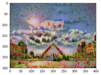

png

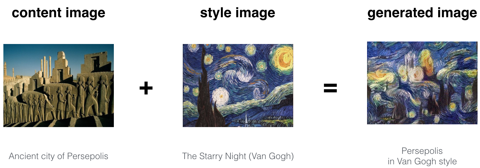
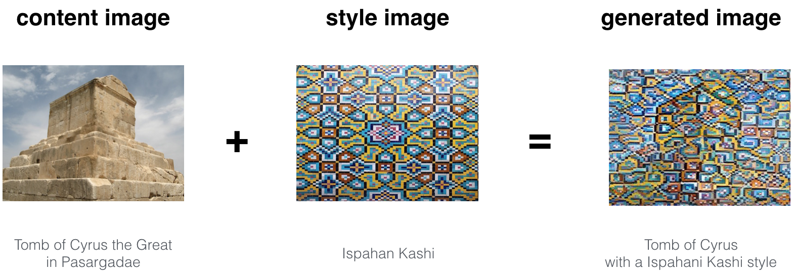
其他的例子:

The beautiful ruins of the ancient city of Persepolis (Iran) with the style of Van Gogh (The Starry Night)
The tomb of Cyrus the great in Pasargadae with the style of a Ceramic Kashi from Ispahan.
A scientific study of a turbulent fluid with the style of a abstract blue fluid painting.

结论

本文介绍了如何对图像进行风格转换，和前面更新神经网络参数不同，这个应用是更新图像的像素值。

风格转换是在给定内容图像和风格图像的基础上，合成新的图像
这个应用使用了实现训练好的神经网络来提取（隐藏层）图像特征
内容代价函数通过隐藏层的输出计算得到
风格函数则是通过计算一个（或多个）隐藏层输出的Gamma矩阵，最终加权求和计算总的风格代价函数
最优化内容和风格代价函数，得到最终合成的新图像

参考资料

吴恩达，coursera深度学习课程
Leon A. Gatys, Alexander S. Ecker, Matthias Bethge, (2015). A Neural Algorithm of Artistic Style (https://arxiv.org/abs/1508.06576)
Harish Narayanan, Convolutional neural networks for artistic style transfer. https://harishnarayanan.org/writing/artistic-style-transfer/
Log0, TensorFlow Implementation of "A Neural Algorithm of Artistic Style". http://www.chioka.in/tensorflow-implementation-neural-algorithm-of-artistic-style
Karen Simonyan and Andrew Zisserman (2015). Very deep convolutional networks for large-scale image recognition (https://arxiv.org/pdf/1409.1556.pdf)
MatConvNet. http://www.vlfeat.org/matconvnet/pretrained/