本章介绍如何使用PySpark进行数据检查、数据清洗、数据统计、数据可视化等工作,并使用一个较大规模的银行诈骗数据作为例子详细介绍这些工具的用法。
数据检查
重复数据
1 | df = spark.createDataFrame([ |
上述数据集有3个问题:
- ID为3有两行而且完全相同
- ID为1和4的两行数据相同(除了ID号不一样以外)
- ID为5有两行但是数据不同
删除完全重复的数据
1 | print('Count of rows: {0}'.format(df.count())) |
Count of rows: 7
Count of distinct row: 6
从上面返回的信息可以知道数据集中存在完全重复的数据。
1 | df = df.dropDuplicates() |
+---+------+------+---+------+
| id|weight|height|age|gender|
+---+------+------+---+------+
|  5| 133.2|   5.7| 54|     F|
|  5| 129.2|   5.3| 42|     M|
|  1| 144.5|   5.9| 33|     M|
|  4| 144.5|   5.9| 33|     M|
|  2| 167.2|   5.4| 45|     M|
|  3| 124.1|   5.2| 23|     F|
+---+------+------+---+------+可以看出\(id=3\)的重复数据已经被删除。
删除内容相同的数据
1 | print('Count of rows: {0}'.format(df.count())) |
Count of rows: 6
Count of distinct ids: 5
1 | df = df.dropDuplicates(subset=[ |
+---+------+------+---+------+
| id|weight|height|age|gender|
+---+------+------+---+------+
|  5| 133.2|   5.7| 54|     F|
|  1| 144.5|   5.9| 33|     M|
|  2| 167.2|   5.4| 45|     M|
|  3| 124.1|   5.2| 23|     F|
|  5| 129.2|   5.3| 42|     M|
+---+------+------+---+------+可以看出,\(id=1\)和\(id=4\)的行合并了。
处理ID编号重复的数据
1 | import pyspark.sql.functions as fn |
+-----+--------+
|count|distance|
+-----+--------+
|    5|       4|
+-----+--------+
可以看出,总共有5行,但是只有4个唯一ID,因此将每一行一个唯一的ID
1 | df.withColumn('new_id', fn.monotonically_increasing_id()).show() |
+---+------+------+---+------+-------------+
| id|weight|height|age|gender|       new_id|
+---+------+------+---+------+-------------+
|  5| 133.2|   5.7| 54|     F|  25769803776|
|  1| 144.5|   5.9| 33|     M| 171798691840|
|  2| 167.2|   5.4| 45|     M| 592705486848|
|  3| 124.1|   5.2| 23|     F|1236950581248|
|  5| 129.2|   5.3| 42|     M|1365799600128|
+---+------+------+---+------+-------------+
当数据放置在不到10亿个分区,每个分区记录少于8亿条时,上面的命令设置的ID号可以保证是唯一的。
未观测数据
1 | df_miss = spark.createDataFrame([ |
+---+------+------+----+------+------+
| id|weight|height| age|gender|income|
+---+------+------+----+------+------+
|  1| 143.5|   5.6|  28|     M|100000|
|  2| 167.2|   5.4|  45|     M|  null|
|  3|  null|   5.2|null|  null|  null|
|  4| 144.5|   5.9|  33|     M|  null|
|  5| 133.2|   5.7|  54|     F|  null|
|  6| 124.1|   5.2|null|     F|  null|
|  7| 129.2|   5.3|  42|     M| 76000|
+---+------+------+----+------+------+
上面的数据集存在以下问题:
- ID为3的行只有一条有用的信息——height
- ID为6的行只缺失一个值——age
- income列的大部分数据是缺失的
- weight和gender列都只缺失一个值
- age列有2个缺失值
查找每行缺少的观测数据
1 | df_miss.rdd.map( |
[(1, 0), (2, 1), (3, 4), (4, 1), (5, 1), (6, 2), (7, 0)]查看\(id=3\)的数据
1 | df_miss.where('id == 3').show() |
+---+------+------+----+------+------+
| id|weight|height| age|gender|income|
+---+------+------+----+------+------+
|  3|  null|   5.2|null|  null|  null|
+---+------+------+----+------+------+
检查每一列中数据缺失的百分比
1 | df_miss.agg(*[ |
+----------+------------------+--------------+------------------+------------------+------------------+
|id_missing|    weight_missing|height_missing|       age_missing|    gender_missing|    income_missing|
+----------+------------------+--------------+------------------+------------------+------------------+
|       0.0|0.1428571428571429|           0.0|0.2857142857142857|0.1428571428571429|0.7142857142857143|
+----------+------------------+--------------+------------------+------------------+------------------+
1 | df_miss.agg(fn.count('weight')).show() |
+-------------+
|count(weight)|
+-------------+
|            6|
+-------------+
处理缺失数据
- 当某一特征缺失严重时,删除这一特征
- 如果数据是离散布尔型,添加新的类别,missing
- 如果是数值型的特征,填充平均数、中间值或者其他的值,可以根据数据分布而定
1 | # 删除income这一个特征 |
1 | # 当某一行数据的特征个数少于3个时,删除这一行数据 |
+---+------+------+----+------+
| id|weight|height| age|gender|
+---+------+------+----+------+
|  1| 143.5|   5.6|  28|     M|
|  2| 167.2|   5.4|  45|     M|
|  4| 144.5|   5.9|  33|     M|
|  5| 133.2|   5.7|  54|     F|
|  6| 124.1|   5.2|null|     F|
|  7| 129.2|   5.3|  42|     M|
+---+------+------+----+------+
1 | means = df_miss_no_income.agg( |
+---+-------------+------+---+-------+
| id|       weight|height|age| gender|
+---+-------------+------+---+-------+
|  1|        143.5|   5.6| 28|      M|
|  2|        167.2|   5.4| 45|      M|
|  3|140.283333333|   5.2| 40|missing|
|  4|        144.5|   5.9| 33|      M|
|  5|        133.2|   5.7| 54|      F|
|  6|        124.1|   5.2| 40|      F|
|  7|        129.2|   5.3| 42|      M|
+---+-------------+------+---+-------+
异常(离群)数据
一种普遍判断该数据是否异常的方法:判断该数据是否落在\([Q1-1.5*IQR, Q3+1.5*IQR]\)范围内,其中\(IQR=Q3-Q1\),\(Q1\)和\(Q3\)分别指上分位和下分位;\(Q1=0.5\)表示是中值;否则认为该数据异常。
1 | df_outliers = spark.createDataFrame([ |
1 | cols = ['weight', 'height', 'age'] |
1 | bounds |
{'age': [-11.0, 93.0],
 'height': [4.499999999999999, 6.1000000000000005],
 'weight': [91.69999999999999, 191.7]}
1 | outliers = df_outliers.select(*['id'] + [ |
+---+--------+--------+-----+
| id|weight_o|height_o|age_o|
+---+--------+--------+-----+
|  1|   false|   false|false|
|  2|   false|   false|false|
|  3|    true|   false| true|
|  4|   false|   false|false|
|  5|   false|   false|false|
|  6|   false|   false|false|
|  7|   false|   false|false|
+---+--------+--------+-----+
1 | bounds |
{'age': [-11.0, 93.0],
 'height': [4.499999999999999, 6.1000000000000005],
 'weight': [91.69999999999999, 191.7]}
1 | df_outliers = df_outliers.join(outliers, on='id') |
+---+------+
| id|weight|
+---+------+
|  3| 342.3|
+---+------+

+---+---+
| id|age|
+---+---+
|  3| 99|
+---+---+
熟悉你的数据
描述性统计
数据加载,并转化为\(DataFrame\)类型
1 | import pyspark.sql.types as typ |
为\(DataFrame\)数据集建立\(schema\)
1 | fields = [ |
创建\(DataFrame\)数据集
1 | fraud_df = spark.createDataFrame(fraud, schema) |
root
 |-- custID: integer (nullable = true)
 |-- gender: integer (nullable = true)
 |-- state: integer (nullable = true)
 |-- cardholder: integer (nullable = true)
 |-- balance: integer (nullable = true)
 |-- numTrans: integer (nullable = true)
 |-- numIntlTrans: integer (nullable = true)
 |-- creditLine: integer (nullable = true)
 |-- fraudRisk: integer (nullable = true)
计算分类列,不同分类的使用频率
1 | fraud_df.groupby('gender').count().show() |
+------+-------+
|gender|  count|
+------+-------+
|     1|6178231|
|     2|3821769|
+------+-------+
从上面可以看出,这是一个类别失衡的数据集(期望的数据集是男女性别数量相同)。
对于数值特征,获取其统计特征:
1 | numerical = ['balance', 'numTrans', 'numIntlTrans'] |
+-------+-----------------+------------------+-----------------+
|summary|          balance|          numTrans|     numIntlTrans|
+-------+-----------------+------------------+-----------------+
|  count|         10000000|          10000000|         10000000|
|   mean|     4109.9199193|        28.9351871|        4.0471899|
| stddev|3996.847309737077|26.553781024522852|8.602970115863767|
|    min|                0|                 0|                0|
|    max|            41485|               100|               60|
+-------+-----------------+------------------+-----------------+
从上面的分析可以看出:
- 所有特征呈正态分布,最大值是平均值的多倍
- 变异系数(均值和标准差之比)非常高(接近或者大于1),表示这是一个数值广泛的特征。
计算偏度
1 | fraud_df.agg({'balance': 'skewness'}).show() |
+------------------+
| skewness(balance)|
+------------------+
|1.1818315552995033|
+------------------+除了\(skewness\)计算偏度以外,还有别的方法
相似性
对\(DataFrame\)数据集计算两个特征之间的相似度十分简单
1 | fraud_df.corr('balance', 'numTrans') |
0.000445231401726595761 | n_numerical = len(numerical) |
[[1.0, 0.00044523140172659576, 0.00027139913398184604],
 [None, 1.0, -0.0002805712819816179],
 [None, None, 1.0]]
数据可视化
1 | %matplotlib inline |
<div class="bk-root">
    <a href="https://bokeh.pydata.org" target="_blank" class="bk-logo bk-logo-small bk-logo-notebook"></a>
    <span id="d9cf94fb-1584-4c53-9d45-c43c04c122ec">Loading BokehJS ...</span>
</div>
直方图
聚集所有工作节点中的数据,返回给驱动程序一个汇总的面元列表和每个面元的计数。
1 | hists = fraud_df.select('balance').rdd.flatMap(lambda row: row).histogram(20) |
1 | data = { |
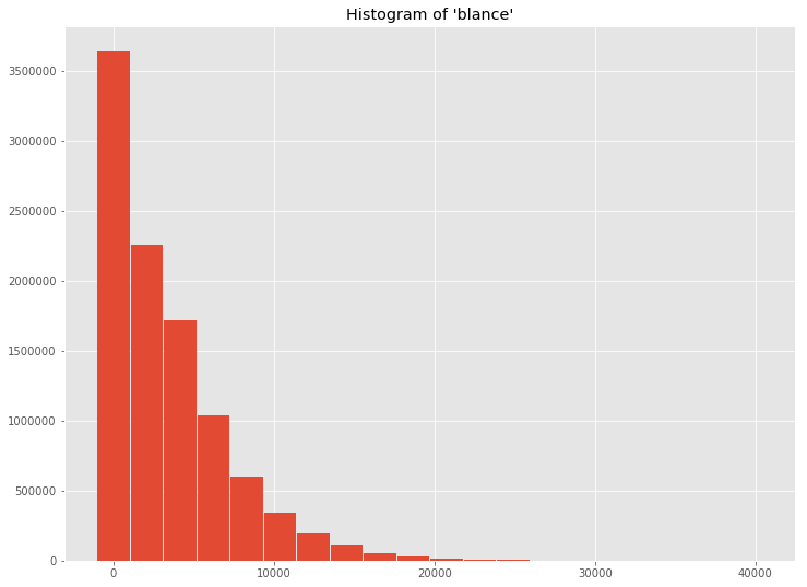
png
用类似的方法,可以用\(Bokeh\)建立直方图
1 | b_hist = chrt.Bar(data, values='freq', label='bins', title='Histogram of \'balance\'') |
如果数据足够小,可以直接使用驱动程序计算直方图
1 | data_driver = { |
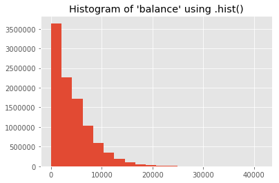
png
1 | b_hist_driver = chrt.Histogram( |
特征之间的交互
随机抽取一部分数据,然后用散点图交互显示不超过3个特征的数据。
1 | data_sample = fraud_df.sampleBy( |
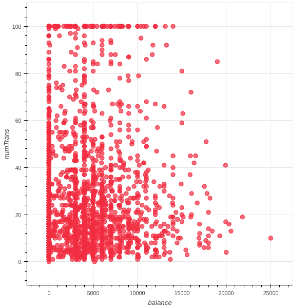
png
小结
- 本问介绍了PySpark中的一些数据分析和清洗的工具,这是机器学习的第一步。
参考资料
- PySpark实战指南,Drabas and Lee著, 栾云杰等译