逻辑回归是机器学习中使用十分广泛的算法,由于它可以看做一层神经网络,因此也是深度学习的基础。本文详细介绍逻辑回归的基本原理及算法实现,最后介绍一个图像识别领域中的猫问题实例。所有内容都是根据吴恩达coursera课程学习整理后得到,详细信息请学习其课程。
基本原理
代价函数
训练样本集为\(\{(x^{(1)},y^{(1)}),(x^{(2)},y^{(2)},...,(x^{(m)},y^{(m)})\}\),其中每一个样本的特征为\(\mathbf{x} \in \mathbb{R}^{n_x}\),\(y \in \{0, 1 \}\)。将\(m\)个训练样本的特征表示为\(\mathbf{X}\in \mathbb{R}^{n_x \times m}\),标签为\(\mathbf{y} \in \mathbb{R}^{1 \times m}\),其中\(n_x\)为特征个数,\(m\)为样本数。
逻辑回归问题可以描述为,寻找最优系数\(\mathbf{W} \in \mathbb{R}^{n_x}\),\(b \in \mathbb{R}\),使得以下代价函数(Cost function)最小: \[ J(\mathbf{W}, b) = \frac{1}{m} \sum_{i=1}^{m} L(\hat{\mathbf{y}}^{(i)},\mathbf{y}^{(i)}) = -\frac{1}{m} \sum_{i=1}^{m} \left[ \mathbf{y}^{(i)} log\hat{\mathbf{y}}^{(i)} + (1-\mathbf{y}^{(i)}) log(1-\hat{\mathbf{y}}^{(i)}) \right] \] 其中\(L(\hat{\mathbf{y}}^{(i)},\mathbf{y}^{(i)})\)表示损失函数。
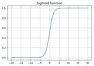
预测值\(\hat{\mathbf{y}}\)通过以下函数预测得到: \[ \hat{\mathbf{y}} = \sigma (\mathbf{W}^T \mathbf{X} + b) \] 其中\(\sigma (\mathbf{z})\)为sigmoid函数, \[ \sigma(\mathbf{z}) = \frac{1}{1+e^{-\mathbf{z}}} \]
1 | import numpy as np |
png
交叉熵代价函数的进一步解释
输入特征向量\(\mathbf{x}\),预测输出\(\hat{y}\): \[ \hat{y} = \sigma(\mathbf{w}^T \mathbf{x} + b) \] 其中\(\sigma(z)=\frac{1}{1+e^{-z}}\)。
预测值\(\hat{y}\)可以解释为结果为1的概率,也就是\(\hat{y} = p(y=1|\mathbf{x})\) \[ If\ y = 1: p(y|\mathbf{x}) = \hat{y} \\ If\ y = 0: p(y|\mathbf{x}) = 1 - \hat{y} \] 上述两式总结为: \[ p(y|\mathbf{x}) = \hat{y}^y (1-\hat{y})^{(1-y)} \] 最大化似然估计函数: \[ log p(y|\mathbf{x}) = y log \hat{y} + (1-y) log (1-\hat{y}) = - L(\hat{y},y) \] 也即最小化交叉熵损失函数。
对\(m\)个样本,最大似然函数为: \[ log p(y^{(1)},...,y^{(m)}) = log \prod_{i=1}^{m} p(y^{(i)}|\mathbf{x}^{(i)}) = - \sum_{i=1}^{m} L(\hat{y}^{(i)}, y^{(i)}) \] 上述公式应用了样本之间独立同分布假设(IDD)。
梯度计算
考虑一个样本两个特征的情况,正过程的计算包括: 1. \(z= w_1 x_1 + w_2 x_2 + b\)
2. \(\hat{y} = a = \sigma(z)\)
3. \(L(a, y) = -[ylog(a) + (1-y) log(1-a)]\)
利用链式法则,反传播过程:
1. \(da = \frac{dL}{da} = -\frac{y}{a}+\frac{1-y}{1-a}\)
2. \(dz = \frac{dL}{da} \frac{da}{dz} = (-\frac{y}{a}+\frac{1-y}{1-a})a(1-a) = a - y\)
3. \(d{w_1} = \frac{dL}{da} \frac{da}{dz} \frac{dz}{dw_1} = x_1 dz\)
\(d{w_2} = x_2 dz\)
\(d{b} = dz\)
扩展到\(m\)个样本,\(n_x\)个特征的情况,正传播过程为: 1. \(\mathbf{z}= \mathbf{W}^T \mathbf{X} + b\)
2. \(\hat{\mathbf{y}} = \mathbf{a} = \sigma(\mathbf{z})\)
3. \(J(\mathbf{a}, \mathbf{y}) = \frac{1}{m} \sum_{i=1}^{m} L(a^{(i)}, y^{(i)}) = -\frac{1}{m} \sum_{i=1}^{m} [y^{(i)}log(a^{(i)}) + (1-y^{(i)}) log(1-a^{(i)})]\)
反传播过程为: 1. \(d\mathbf{a} =\frac{dJ}{d\mathbf{a}} = -\frac{1}{m} \left[ \frac{\mathbf{y}}{\mathbf{a}}+\frac{1-\mathbf{y}}{1-\mathbf{a}} \right]\)
2. \(d\mathbf{z} = \frac{1}{m} (\mathbf{a} - \mathbf{y})\)
3. \(d\mathbf{w} = \mathbf{X} d\mathbf{z}^T = \frac{1}{m} \mathbf{X} (\mathbf{a} - \mathbf{y})^T\)
\(db = \frac{1}{m} \sum_{i=1}^{m} dz^{(i)}\)
算法实现
向量化:任何情况都尽量避免使用\(for\)循环,而是使用\(numpy\)库中的矩阵运算;
广播功能:对于矩阵运算,一种十分方便的功能是广播,可以自动对维度进行扩展;
尽量指定矩阵维度信息,而最好不要用秩为1的数组;
多采用\(assert\)函数检查维度信息;
也可以使用\(reshape\)函数重新整形数组结构
向量化
任何情况都尽量避免使用\(for\)循环,而是使用\(numpy\)库中的矩阵运算;
1 | %%time |
y= [ 99767.80813156]
CPU times: user 530 ms, sys: 71 µs, total: 530 ms
Wall time: 531 ms
1 | %%time |
y= [[ 99527.05123125]]
CPU times: user 5.73 ms, sys: 3.47 ms, total: 9.2 ms
Wall time: 7.62 ms可以看出,使用\(numpy\)库中的向量化实现,速度快了很多。
1 | np.random.randn? |
广播功能
下面以softmax函数为例介绍python的广播功能,softmax函数在多分类问题中经常使用,具体的公式如下:
- $ x ^{1n} softmax(x) = softmax(
\[\begin{bmatrix}
x_1 &&
x_2 &&
... &&
x_n
\end{bmatrix}\]
) =
\[\begin{bmatrix}
\frac{e^{x_1}}{\sum_{j}e^{x_j}} &&
\frac{e^{x_2}}{\sum_{j}e^{x_j}} &&
... &&
\frac{e^{x_n}}{\sum_{j}e^{x_j}}
\end{bmatrix}\]
$
\(\text{for a matrix } x \in \mathbb{R}^{m \times n} \text{, $x_{ij}$ maps to the element in the $i^{th}$ row and $j^{th}$ column of $x$, thus we have: }\) \[softmax(x) = softmax\begin{bmatrix} x_{11} & x_{12} & x_{13} & \dots & x_{1n} \\ x_{21} & x_{22} & x_{23} & \dots & x_{2n} \\ \vdots & \vdots & \vdots & \ddots & \vdots \\ x_{m1} & x_{m2} & x_{m3} & \dots & x_{mn} \end{bmatrix} = \begin{bmatrix} \frac{e^{x_{11}}}{\sum_{j}e^{x_{1j}}} & \frac{e^{x_{12}}}{\sum_{j}e^{x_{1j}}} & \frac{e^{x_{13}}}{\sum_{j}e^{x_{1j}}} & \dots & \frac{e^{x_{1n}}}{\sum_{j}e^{x_{1j}}} \\ \frac{e^{x_{21}}}{\sum_{j}e^{x_{2j}}} & \frac{e^{x_{22}}}{\sum_{j}e^{x_{2j}}} & \frac{e^{x_{23}}}{\sum_{j}e^{x_{2j}}} & \dots & \frac{e^{x_{2n}}}{\sum_{j}e^{x_{2j}}} \\ \vdots & \vdots & \vdots & \ddots & \vdots \\ \frac{e^{x_{m1}}}{\sum_{j}e^{x_{mj}}} & \frac{e^{x_{m2}}}{\sum_{j}e^{x_{mj}}} & \frac{e^{x_{m3}}}{\sum_{j}e^{x_{mj}}} & \dots & \frac{e^{x_{mn}}}{\sum_{j}e^{x_{mj}}} \end{bmatrix} = \begin{pmatrix} softmax\text{(first row of x)} \\ softmax\text{(second row of x)} \\ ... \\ softmax\text{(last row of x)} \\ \end{pmatrix} \]
1 | # GRADED FUNCTION: softmax |
1 | x = np.array([ |
softmax(x) = [[  9.80897665e-01   8.94462891e-04   1.79657674e-02   1.21052389e-04
    1.21052389e-04]
 [  8.78679856e-01   1.18916387e-01   8.01252314e-04   8.01252314e-04
    8.01252314e-04]]
实例
下面介绍如何使用逻辑回归对图片进行分类,判断是否是猫的图片。
加载数据
数据格式为h5,需要安装h5py库进行读取,原始数据中特征的维度为(m, num_px, num_px, 3),输出y的维度为(1, m)。为了保持和前面原理部分一致,需要reshape数据为(num_pxnum_px3, m)。
1 | import numpy as np |
1 | # Loading the data (cat/non-cat) |
y = [1], it's a 'cat' picture.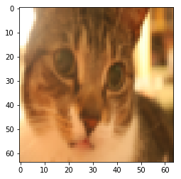
png
1 | ### START CODE HERE ### (≈ 3 lines of code) |
Number of training examples: m_train = 209
Number of testing examples: m_test = 50
Height/Width of each image: num_px = 64
Each image is of size: (64, 64, 3)
train_set_x shape: (209, 64, 64, 3)
train_set_y shape: (1, 209)
test_set_x shape: (50, 64, 64, 3)
test_set_y shape: (1, 50)
1 | # Reshape the training and test examples |
train_set_x_flatten shape: (12288, 209)
train_set_y shape: (1, 209)
test_set_x_flatten shape: (12288, 50)
test_set_y shape: (1, 50)
sanity check after reshaping: [17 31 56 22 33]
预处理数据
彩色图像中每个像素点包含3个特征(RGB),每个特征取值范围从0到255。
在机器学习中,通用的预处理步骤中需要对数据进行中心化和标准化,也就是说:每个样本减掉所有样本的均值,并除以所有样本的标准差。但是对于图像数据,一种更加简单和方便的做法是对数据集除以255,这种做法和通用的做法效果相当。
1 | train_set_x = train_set_x_flatten/255. |
学习算法
逻辑回归实际上是一个非常简单的神经网络学习算法,如下图所示
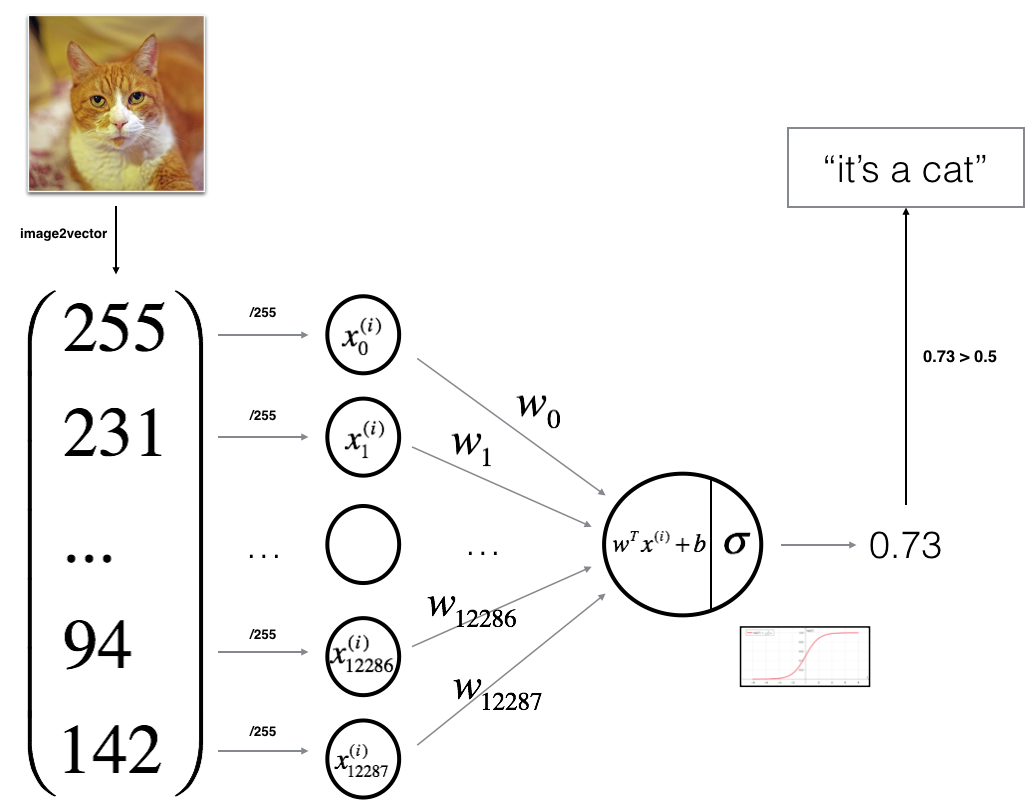
该算法的数学表达式为:
对一个样本 \(x^{(i)}\): \[z^{(i)} = w^T x^{(i)} + b \tag{1}\] \[\hat{y}^{(i)} = a^{(i)} = sigmoid(z^{(i)})\tag{2}\] \[ \mathcal{L}(a^{(i)}, y^{(i)}) = - y^{(i)} \log(a^{(i)}) - (1-y^{(i)} ) \log(1-a^{(i)})\tag{3}\]
代价函数为所有训练样本的损失函数之和: \[ J = \frac{1}{m} \sum_{i=1}^m \mathcal{L}(a^{(i)}, y^{(i)})\tag{6}\]
关键步骤: - 模型参数化 - 通过最小化代价函数学习参数 - 利用学习的参数对测试数据进行预测 - 分析结果
建立一个神经网络的主要步骤是: 1. 定义网络结构(例如输入特征的数量、层数、神经元个数等) 2. 模型参数初始化 3. 循环: - 计算当前损失函数(正传) - 计算当前梯度(反传) - 更新模型参数(梯度下降法)
1 | # GRADED FUNCTION: sigmoid |
1 | print ("sigmoid([0, 2]) = " + str(sigmoid(np.array([0,2])))) |
sigmoid([0, 2]) = [ 0.5 0.88079708]1 | # GRADED FUNCTION: initialize_with_zeros |
1 | dim = 2 |
w = [[ 0.]
 [ 0.]]
b = 0
正传过程: - You get X - You compute \(A = \sigma(w^T X + b) = (a^{(0)}, a^{(1)}, ..., a^{(m-1)}, a^{(m)})\) - You calculate the cost function: \(J = -\frac{1}{m}\sum_{i=1}^{m}y^{(i)}\log(a^{(i)})+(1-y^{(i)})\log(1-a^{(i)})\)
反传必须要用到的公式:
\[ \frac{\partial J}{\partial w} = \frac{1}{m}X(A-Y)^T\tag{7}\] \[ \frac{\partial J}{\partial b} = \frac{1}{m} \sum_{i=1}^m (a^{(i)}-y^{(i)})\tag{8}\]
1 | # GRADED FUNCTION: propagate |
1 | w, b, X, Y = np.array([[1],[2]]), 2, np.array([[1,2],[3,4]]), np.array([[1,0]]) |
dw = [[ 0.99993216]
 [ 1.99980262]]
db = [ 0.49993523]
cost = 6.000064773192205
最优化过程: - 初始化参数 - 计算代价函数和梯度 - 利用梯度下降法更新参数 对参数\(\theta\), 更新的法则是$ = - d$, 其中 \(\alpha\) 是学习率.
1 | # GRADED FUNCTION: optimize |
1 | params, grads, costs = optimize(w, b, X, Y, num_iterations= 100, learning_rate = 0.009, print_cost = False) |
w = [[ 0.1124579 ]
 [ 0.23106775]]
b = [ 1.55930492]
dw = [[ 0.90158428]
 [ 1.76250842]]
db = [ 0.43046207]
预测过程: 1. 计算\(\hat{Y} = A = \sigma(w^T X + b)\)
2. 将输出转化为0 (if activation <= 0.5) 或 1 (if activation > 0.5)
1 | # GRADED FUNCTION: predict |
1 | print ("predictions = " + str(predict(w, b, X))) |
predictions = [[ 1. 1.]]将所有的函数合并成一个model函数
1 | # GRADED FUNCTION: model |
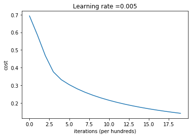
1 | d = model(train_set_x, train_set_y, test_set_x, test_set_y, num_iterations = 2000, learning_rate = 0.005, print_cost = True) |
Cost after iteration 0: 0.693147
Cost after iteration 100: 0.584508
Cost after iteration 200: 0.466949
Cost after iteration 300: 0.376007
Cost after iteration 400: 0.331463
Cost after iteration 500: 0.303273
Cost after iteration 600: 0.279880
Cost after iteration 700: 0.260042
Cost after iteration 800: 0.242941
Cost after iteration 900: 0.228004
Cost after iteration 1000: 0.214820
Cost after iteration 1100: 0.203078
Cost after iteration 1200: 0.192544
Cost after iteration 1300: 0.183033
Cost after iteration 1400: 0.174399
Cost after iteration 1500: 0.166521
Cost after iteration 1600: 0.159305
Cost after iteration 1700: 0.152667
Cost after iteration 1800: 0.146542
Cost after iteration 1900: 0.140872
train accuracy: 99.04306220095694 %
test accuracy: 70.0 %
从结果可以看出,该模型过拟合。需要进一步采用正则化或者其他手段解决这个问题。
1 | # Example of a picture that was wrongly classified. |
y = 1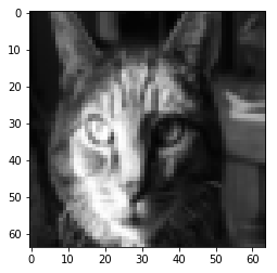
png
1 | # Plot learning curve (with costs) |
png
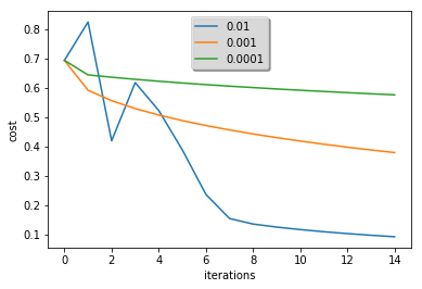
1 | learning_rates = [0.01, 0.001, 0.0001] |
learning rate is: 0.01
train accuracy: 99.52153110047847 %
test accuracy: 68.0 %

-------------------------------------------------------

learning rate is: 0.001
train accuracy: 88.99521531100478 %
test accuracy: 64.0 %

-------------------------------------------------------

learning rate is: 0.0001
train accuracy: 68.42105263157895 %
test accuracy: 36.0 %

-------------------------------------------------------
png
1 | ## START CODE HERE ## (PUT YOUR IMAGE NAME) |
y = 0.0, your algorithm predicts a "non-cat" picture.
png
小结
- 逻辑回归是机器学习领域的基础算法,也是深度神经网路的基础
- 图像的预处理十分关键
- 完整的介绍了逻辑回归的实现流程,同样可以扩展到深度神经网络的实现
参考资料
- 吴恩达,coursera深度学习课程