本文实现一个将文本转化成表情包的模型。由于使用了词编码模型,尽管使用很少的训练数据,也可以准确的将没有出现的词汇映射到相同的表情包上。本文先从一个简单的模型(Emojifier-V1)出发,介绍词嵌入模型的用法,然后引入LSTM模型,改进为可以利用上下文信息的更加先进的表情包模型。
1 | import numpy as np |
基础模型:Emojifier-V1
EMOJISET数据集
首先,使用一个小的数据集,建立一个简单的基础模型:
- X包含127个句子
- Y包含0到4的整型标签,每个数字对应一个表情
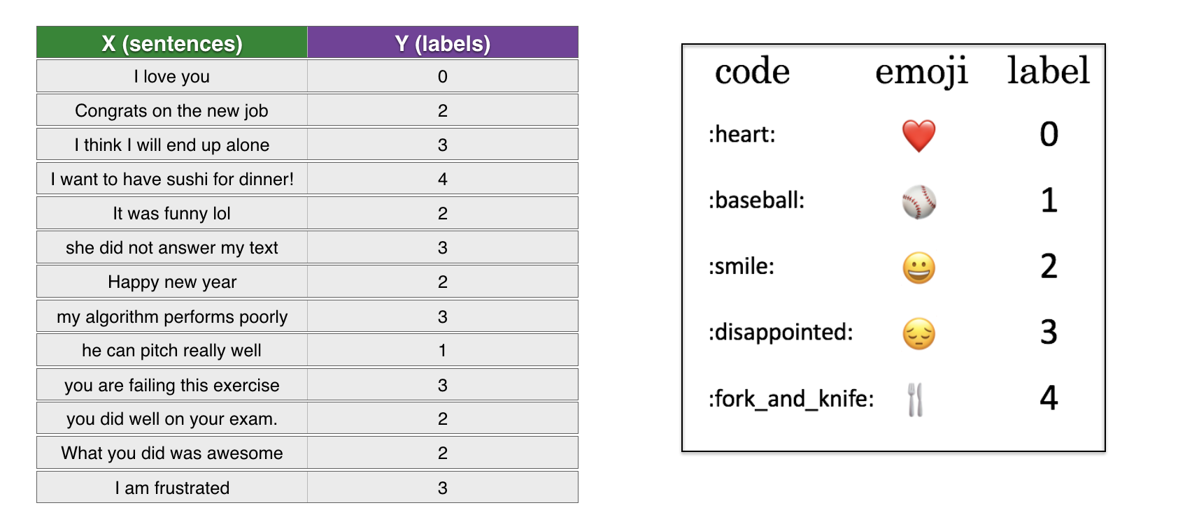
下面加载数据集,并分为训练集(127个样本)和测试集(56个样本)。
1 | X_train, Y_train = read_csv('data/emoji_data/train_emoji.csv') |
1 | maxLen = len(max(X_train, key=len).split()) |
1 | index = 1 |
I am proud of your achievements 😄Emojifier-V1简介
下面实现基本模型Emojifier-v1:
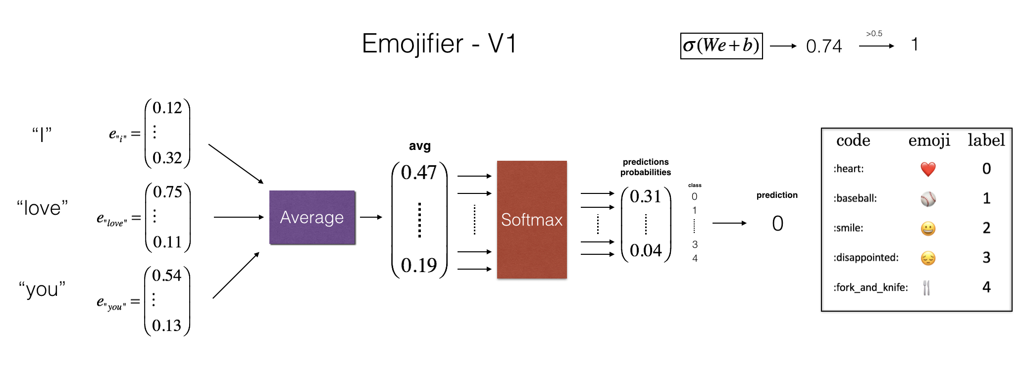
模型的输入是句子(也就是字符串,比如"I love you")。输出是形状为(1,5)的概率向量,输入argmax层输出最有可能的表情。
1 | Y_oh_train = convert_to_one_hot(Y_train, C = 5) |
1 | index = 50 |
0 is converted into one hot [ 1. 0. 0. 0. 0.]实现Emojifier-V1
如图(2)所示,第一步是将输入的句子转化为词向量,然后取平均。这里使用首先训练好的50维GloVe编码模型获取词向量。
1 | word_to_index, index_to_word, word_to_vec_map = read_glove_vecs('model_data/glove.6B.50d.txt') |
加载后得到:
- word_to_index: 单词映射到单词表(400,001个单词,有效的索引范围0-400,000)索引的字典.
- index_to_word: 索引映射到单词
- word_to_vec_map: 单词映射到GloVe词向量
运行下面的单元,验证是否有效。
1 | word = "cucumber" |
the index of cucumber in the vocabulary is 113317
the 289846th word in the vocabulary is potatos下面实现sentence_to_avg(),包括两步:
1. 将所有的句子转化为小写,然后分割为词序列。参考X.lower()和X.split()
2. 对句子中的每个单词,获取它的GloVe词嵌入表示。然后进行平均
1 | # GRADED FUNCTION: sentence_to_avg |
1 | avg = sentence_to_avg("Morrocan couscous is my favorite dish", word_to_vec_map) |
avg =  [-0.008005    0.56370833 -0.50427333  0.258865    0.55131103  0.03104983
 -0.21013718  0.16893933 -0.09590267  0.141784   -0.15708967  0.18525867
  0.6495785   0.38371117  0.21102167  0.11301667  0.02613967  0.26037767
  0.05820667 -0.01578167 -0.12078833 -0.02471267  0.4128455   0.5152061
  0.38756167 -0.898661   -0.535145    0.33501167  0.68806933 -0.2156265
  1.797155    0.10476933 -0.36775333  0.750785    0.10282583  0.348925
 -0.27262833  0.66768    -0.10706167 -0.283635    0.59580117  0.28747333
 -0.3366635   0.23393817  0.34349183  0.178405    0.1166155  -0.076433
  0.1445417   0.09808667]
计算句子的词嵌入平均之后,正传,然后计算损失函数,反传更新softmax层的参数。需要实现的公式包括:
\[ z^{(i)} = W . avg^{(i)} + b\] \[ a^{(i)} = softmax(z^{(i)})\] \[ \mathcal{L}^{(i)} = - \sum_{k = 0}^{n_y - 1} Yoh^{(i)}_k * log(a^{(i)}_k)\]
1 | # GRADED FUNCTION: model |
1 | print(X_train.shape) |
(132,)
(132,)
(132, 5)
never talk to me again
<class 'numpy.ndarray'>
(20,)
(20,)
(132, 5)
<class 'numpy.ndarray'>
运行下面的计算单元,训练模型,并更新softmax层参数
1 | pred, W, b = model(X_train, Y_train, word_to_vec_map) |
Epoch: 0 --- cost = 1.95204988128
Accuracy: 0.348484848485
Epoch: 100 --- cost = 0.0797181872601
Accuracy: 0.931818181818
Epoch: 200 --- cost = 0.0445636924368
Accuracy: 0.954545454545
Epoch: 300 --- cost = 0.0343226737879
Accuracy: 0.969696969697
[[ 3.]
 [ 2.]
 [ 3.]
 [ 0.]
 [ 4.]
 [ 0.]
 [ 3.]
 [ 2.]
 [ 3.]
 [ 1.]
 [ 3.]
 [ 3.]
 [ 1.]
 [ 3.]
 [ 2.]
 [ 3.]
 [ 2.]
 [ 3.]
 [ 1.]
 [ 2.]
 [ 3.]
 [ 0.]
 [ 2.]
 [ 2.]
 [ 2.]
 [ 1.]
 [ 4.]
 [ 3.]
 [ 3.]
 [ 4.]
 [ 0.]
 [ 3.]
 [ 4.]
 [ 2.]
 [ 0.]
 [ 3.]
 [ 2.]
 [ 2.]
 [ 3.]
 [ 4.]
 [ 2.]
 [ 2.]
 [ 0.]
 [ 2.]
 [ 3.]
 [ 0.]
 [ 3.]
 [ 2.]
 [ 4.]
 [ 3.]
 [ 0.]
 [ 3.]
 [ 3.]
 [ 3.]
 [ 4.]
 [ 2.]
 [ 1.]
 [ 1.]
 [ 1.]
 [ 2.]
 [ 3.]
 [ 1.]
 [ 0.]
 [ 0.]
 [ 0.]
 [ 3.]
 [ 4.]
 [ 4.]
 [ 2.]
 [ 2.]
 [ 1.]
 [ 2.]
 [ 0.]
 [ 3.]
 [ 2.]
 [ 2.]
 [ 0.]
 [ 3.]
 [ 3.]
 [ 1.]
 [ 2.]
 [ 1.]
 [ 2.]
 [ 2.]
 [ 4.]
 [ 3.]
 [ 3.]
 [ 2.]
 [ 4.]
 [ 0.]
 [ 0.]
 [ 3.]
 [ 3.]
 [ 3.]
 [ 3.]
 [ 2.]
 [ 0.]
 [ 1.]
 [ 2.]
 [ 3.]
 [ 0.]
 [ 2.]
 [ 2.]
 [ 2.]
 [ 3.]
 [ 2.]
 [ 2.]
 [ 2.]
 [ 4.]
 [ 1.]
 [ 1.]
 [ 3.]
 [ 3.]
 [ 4.]
 [ 1.]
 [ 2.]
 [ 1.]
 [ 1.]
 [ 3.]
 [ 1.]
 [ 0.]
 [ 4.]
 [ 0.]
 [ 3.]
 [ 3.]
 [ 4.]
 [ 4.]
 [ 1.]
 [ 4.]
 [ 3.]
 [ 0.]
 [ 2.]]
检查测试集的性能
1 | print("Training set:") |
Training set:
Accuracy: 0.977272727273
Test set:
Accuracy: 0.857142857143如果随机猜的话,只有20%的准确率,但是这里只需要127个样本,就可以达到这么好的性能。在训练集中,算法见过类似于"I love you"这样的句子,并标定为 ❤️。而"adore"没有在训练集出现过,下面看看"I adore you."会出来什么?
1 | X_my_sentences = np.array(["i adore you", "i love you", "funny lol", "lets play with a ball", "food is ready", "not feeling happy"]) |
Accuracy: 0.833333333333

i adore you ❤️
i love you ❤️
funny lol 😄
lets play with a ball ⚾
food is ready 🍴
not feeling happy 😄
结果十分令人惊讶!这是因为"adore"和"love"具有类似的词嵌入,这个算法可以很好地泛化到训练集中没有出现过的单词。
但是这个算法不能理解"not feeling happy"。这是因为它忽略了词的顺序。
打印出混淆矩阵可以帮助我们理解哪些类别更难标定。混淆矩阵显示的是算法将真实的类别错误的划分为另一个类别的概率。
1 | print(Y_test.shape) |
(56,)
           ❤️    ⚾    😄    😞   🍴
Predicted  0.0  1.0  2.0  3.0  4.0  All
Actual
0            6    0    0    1    0    7
1            0    8    0    0    0    8
2            2    0   16    0    0   18
3            1    1    2   12    0   16
4            0    0    1    0    6    7
All          9    9   19   13    6   56
png
从上面的例子可以看出:
- 尽管只有127个训练样本,但是仍然可以获得比较好的表情模型,主要是因为词向量带来的泛化能力
- Emojify-V1在形如"This movie is not good and not enjoyable"的句子表现不好,是因为它不能理解词的组合,仅仅是平均所有的词嵌入向量,没有注意词的顺序。下面将介绍一个性能更好的模型
Emojifier-V2:使用Keras中的LSTM层
下面建立一个LSTM模型,它将输入单词序列作为输入。这个模型能够将单词顺序考虑进去。Emojifier-V2也使用预训练好的词嵌入模型,但是将其输入到LSTM层中,预测最有可能的表情。
1 | import numpy as np |
Using TensorFlow backend.模型概述
下面是Emojifier-v2模型的示意图: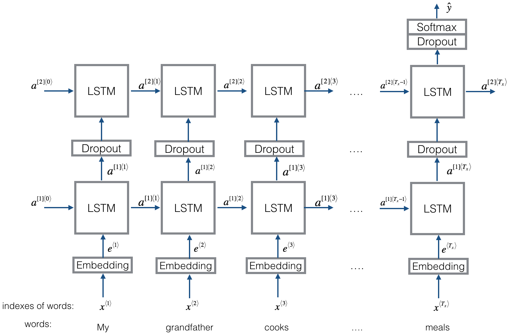
Keras和mini-batching
在大多数深度学习框架中,相同的mini-batch中所有的序列长度相同,这样才可以向量化。如果一个句子有3个词,另一个句子有4个词,那么它们的计算量不一样(一个需要3步LSTM、一个需要4步LSTM,无法同时计算。
最常见的做法是使用补零。具体的,设置最长的序列长度,然后将所有的句子补到这么长。例如,设置最长的序列长度为20,我们可以让每个句子补零,使得每个输入的句子长度都为20.因此,像 "i love you"这样的句子就变成\((e_{i}, e_{love}, e_{you}, \vec{0}, \vec{0}, \ldots, \vec{0})\)。而任何长于20个单词的句子则会截断。
词嵌入层
在Keras中,词嵌入矩阵表示为一个层,并将一些列正实数(单词所对应的下标)映射为固定长度的向量(词嵌入向量)。该矩阵一般是预训练好了的。本文将介绍在Keras中如何创建Embedding()层,并将其初始化为之前加载过的GloVe 50维的词向量。由于我们的训练集很小,因此不会更新词嵌入模型,而是将其固定。但是下面的代码会显示如何训练以及固定词嵌入层。
Embedding()层输入一个整数矩阵,大小为(batch size, max input length)。代表的是句子转化为索引列表。如下图所示:
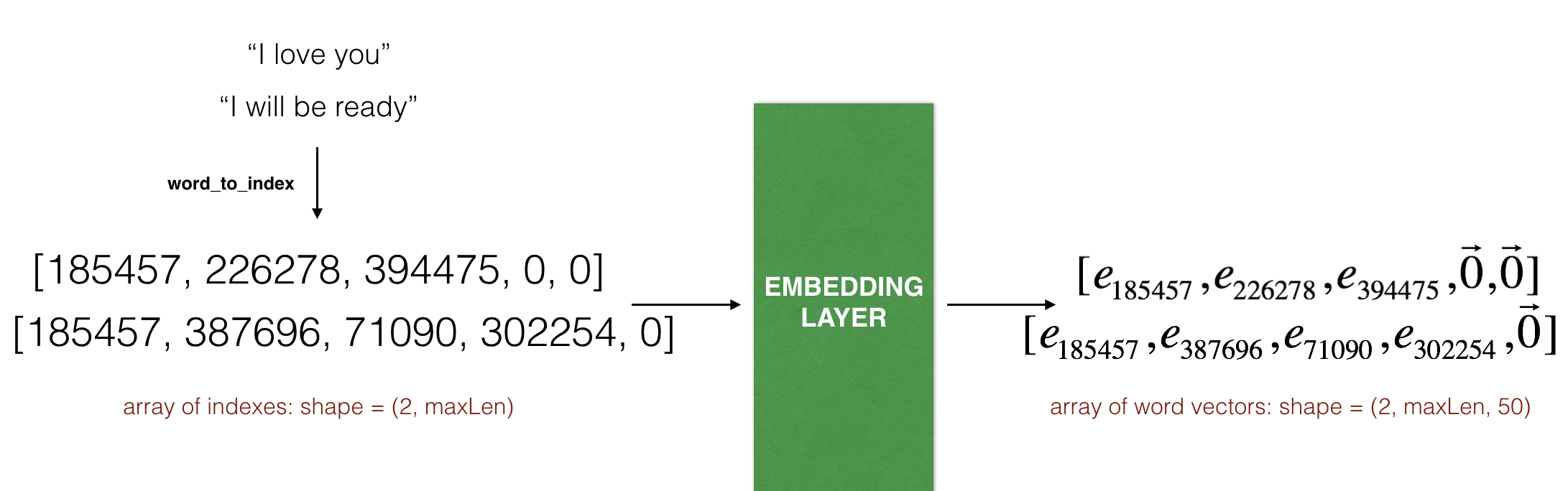
max_len=5。最后的输出为(2,max_len,50).
1 | # GRADED FUNCTION: sentences_to_indices |
下面测试sentences_to_indices()
1 | X1 = np.array(["funny lol", "lets play baseball", "food is ready for you"]) |
X1 = ['funny lol' 'lets play baseball' 'food is ready for you']
X1_indices = [[ 155345.  225122.       0.       0.       0.]
 [ 220930.  286375.   69714.       0.       0.]
[ 151204. 192973. 302254. 151349. 394475.]]下面在Keras中用预训练好的词向量构建Embedding()层。当这些层已经构建了之后,sentences_to_indices()的输出作为词嵌入层的输入,最后返回该句子的词嵌入向量。
实现pretrained_embedding_layer()函数包括:
- 以正确的维度零初始化词嵌入矩阵
- 把所有从word_to_vec_map提取的词嵌入向量填入词嵌入矩阵
- 定义Keras词嵌入层。使用Embedding(),确保这一层不是可训练层。如果设置trainable = True,那么优化算法会修改词嵌入表示
- 设置词嵌入权值等于词嵌入矩阵
1 | # GRADED FUNCTION: pretrained_embedding_layer |
1 | embedding_layer = pretrained_embedding_layer(word_to_vec_map, word_to_index) |
weights[0][1][3] = -0.3403建立Emojifier-V2模型
使用上面建立的词嵌入层,将其输出作为LSTM网络的输入。
模型的输入为句子序列,维度为(m, max_len, ),输出为softmax概率向量,维度为(m, C = 5)。需要用到的Keras函数有:
Input(shape = ..., dtype = '...'), LSTM(), Dropout(), Dense(), 和 Activation().
1 | # GRADED FUNCTION: Emojify_V2 |
1 | model = Emojify_V2((maxLen,), word_to_vec_map, word_to_index) |
WARNING:tensorflow:From /home/seisinv/anaconda3/envs/fwi_ai/lib/python3.5/site-packages/keras/backend/tensorflow_backend.py:1190: calling reduce_sum (from tensorflow.python.ops.math_ops) with keep_dims is deprecated and will be removed in a future version.
Instructions for updating:
keep_dims is deprecated, use keepdims instead
_________________________________________________________________
Layer (type)                 Output Shape              Param #
=================================================================
input_1 (InputLayer)         (None, 10)                0
_________________________________________________________________
embedding_2 (Embedding)      (None, 10, 50)            20000050
_________________________________________________________________
lstm_1 (LSTM)                (None, 10, 128)           91648
_________________________________________________________________
dropout_1 (Dropout)          (None, 10, 128)           0
_________________________________________________________________
lstm_2 (LSTM)                (None, 128)               131584
_________________________________________________________________
dropout_2 (Dropout)          (None, 128)               0
_________________________________________________________________
dense_1 (Dense)              (None, 5)                 645
_________________________________________________________________
activation_1 (Activation)    (None, 5)                 0
=================================================================
Total params: 20,223,927
Trainable params: 20,223,927
Non-trainable params: 0
_________________________________________________________________
1 | model.compile(loss='categorical_crossentropy', optimizer='adam', metrics=['accuracy']) |
WARNING:tensorflow:From /home/seisinv/anaconda3/envs/fwi_ai/lib/python3.5/site-packages/keras/backend/tensorflow_backend.py:1297: calling reduce_mean (from tensorflow.python.ops.math_ops) with keep_dims is deprecated and will be removed in a future version.
Instructions for updating:
keep_dims is deprecated, use keepdims instead
1 | X_train_indices = sentences_to_indices(X_train, word_to_index, maxLen) |
1 | model.fit(X_train_indices, Y_train_oh, epochs = 50, batch_size = 32, shuffle=True) |
Epoch 1/50
132/132 [==============================] - 5s - loss: 1.6086 - acc: 0.1667
Epoch 2/50
132/132 [==============================] - 1s - loss: 1.5876 - acc: 0.3333
Epoch 3/50
132/132 [==============================] - 1s - loss: 1.5725 - acc: 0.2652
Epoch 4/50
132/132 [==============================] - 1s - loss: 1.5532 - acc: 0.3485
Epoch 5/50
132/132 [==============================] - 1s - loss: 1.5397 - acc: 0.3030
Epoch 6/50
132/132 [==============================] - 1s - loss: 1.5155 - acc: 0.3712
Epoch 7/50
132/132 [==============================] - 1s - loss: 1.5170 - acc: 0.3409
Epoch 8/50
132/132 [==============================] - 1s - loss: 1.4453 - acc: 0.4848
Epoch 9/50
132/132 [==============================] - 1s - loss: 1.4056 - acc: 0.5152
Epoch 10/50
132/132 [==============================] - 1s - loss: 1.3391 - acc: 0.6515
Epoch 11/50
132/132 [==============================] - 1s - loss: 1.2934 - acc: 0.6439
Epoch 12/50
132/132 [==============================] - 1s - loss: 1.2247 - acc: 0.7273
Epoch 13/50
132/132 [==============================] - 1s - loss: 1.1986 - acc: 0.7727
Epoch 14/50
132/132 [==============================] - 1s - loss: 1.1831 - acc: 0.7500
Epoch 15/50
132/132 [==============================] - 1s - loss: 1.1318 - acc: 0.8258
Epoch 16/50
132/132 [==============================] - 1s - loss: 1.1317 - acc: 0.7955
Epoch 17/50
132/132 [==============================] - 1s - loss: 1.0946 - acc: 0.8182
Epoch 18/50
132/132 [==============================] - 1s - loss: 1.0895 - acc: 0.8258
Epoch 19/50
132/132 [==============================] - 1s - loss: 1.0386 - acc: 0.8864
Epoch 20/50
132/132 [==============================] - 1s - loss: 1.0398 - acc: 0.8561
Epoch 21/50
132/132 [==============================] - 2s - loss: 1.0059 - acc: 0.9091
Epoch 22/50
132/132 [==============================] - 2s - loss: 1.0045 - acc: 0.9015
Epoch 23/50
132/132 [==============================] - 2s - loss: 0.9920 - acc: 0.9394
Epoch 24/50
132/132 [==============================] - 2s - loss: 0.9754 - acc: 0.9394
Epoch 25/50
132/132 [==============================] - 2s - loss: 0.9598 - acc: 0.9545
Epoch 26/50
132/132 [==============================] - 2s - loss: 0.9453 - acc: 0.9697
Epoch 27/50
132/132 [==============================] - 2s - loss: 0.9460 - acc: 0.9621
Epoch 28/50
132/132 [==============================] - 2s - loss: 0.9378 - acc: 0.9697
Epoch 29/50
132/132 [==============================] - 2s - loss: 0.9406 - acc: 0.9697
Epoch 30/50
132/132 [==============================] - 2s - loss: 0.9395 - acc: 0.9697
Epoch 31/50
132/132 [==============================] - 2s - loss: 0.9388 - acc: 0.9697
Epoch 32/50
132/132 [==============================] - 2s - loss: 0.9382 - acc: 0.9621
Epoch 33/50
132/132 [==============================] - 2s - loss: 0.9316 - acc: 0.9773
Epoch 34/50
132/132 [==============================] - 2s - loss: 0.9335 - acc: 0.9697
Epoch 35/50
132/132 [==============================] - 2s - loss: 0.9312 - acc: 0.9773
Epoch 36/50
132/132 [==============================] - 2s - loss: 0.9457 - acc: 0.9621
Epoch 37/50
132/132 [==============================] - 2s - loss: 0.9287 - acc: 0.9773
Epoch 38/50
132/132 [==============================] - 2s - loss: 0.9353 - acc: 0.9697
Epoch 39/50
132/132 [==============================] - 2s - loss: 0.9328 - acc: 0.9697
Epoch 40/50
132/132 [==============================] - 2s - loss: 0.9281 - acc: 0.9773
Epoch 41/50
132/132 [==============================] - 2s - loss: 0.9314 - acc: 0.9773
Epoch 42/50
132/132 [==============================] - 2s - loss: 0.9325 - acc: 0.9697
Epoch 43/50
132/132 [==============================] - 1s - loss: 0.9356 - acc: 0.9697
Epoch 44/50
132/132 [==============================] - 1s - loss: 0.9281 - acc: 0.9773
Epoch 45/50
132/132 [==============================] - 1s - loss: 0.9285 - acc: 0.9773
Epoch 46/50
132/132 [==============================] - 1s - loss: 0.9280 - acc: 0.9773
Epoch 47/50
132/132 [==============================] - 1s - loss: 0.9271 - acc: 0.9773
Epoch 48/50
132/132 [==============================] - 1s - loss: 0.9292 - acc: 0.9773
Epoch 49/50
132/132 [==============================] - 1s - loss: 0.9334 - acc: 0.9697
Epoch 50/50
132/132 [==============================] - 1s - loss: 0.9632 - acc: 0.9242


<keras.callbacks.History at 0x7faab0bbad30>
测试集
1 | X_test_indices = sentences_to_indices(X_test, word_to_index, max_len = maxLen) |
32/56 [================>.............] - ETA: 0s
Test accuracy =  0.857142848628
1 | # This code allows you to see the mislabelled examples |
Expected emoji:😄 prediction: he got a very nice raise   😞
Expected emoji:😄 prediction: she got me a nice present  😞
Expected emoji:😄 prediction: Stop making this joke ha ha ha 😞
Expected emoji:😄 prediction: you brighten my day    ❤️
Expected emoji:😄 prediction: will you be my valentine   ❤️
Expected emoji:🍴 prediction: I am hungry😞
Expected emoji:😄 prediction: What you did was awesome   😞
Expected emoji:😞 prediction: go away    ⚾
1 | # Change the sentence below to see your prediction. Make sure all the words are in the Glove embeddings. |
not feeling happy 😞从上面的例子可以看出,使用LSTM可以部分解决第一个版本的问题,但是对类似于"not happy"这样的句子表现仍然不是很好,这是因为训练集太小,没有太多的负例。
小结
- 在NLP任务中,如果你的训练集很小,使用词嵌入可以极大地改善算法性能。词嵌入允许你的模型对训练集没有出现过的样例也工作良好。
- 在Keras中训练序列模型需要注意以下几点:
-- 为了使用mini-batch,要将序列补零,以使得在mini-batch中所有样例长度相同
--Embedding()层可以使用与训练好的模型进行初始化,也可以进一步使用你的数据集进一步训练。但是,如果带标签的训练集很小,通常没有必要再训练词嵌入模型
--LSTM()层有一个参数return_sequences,表示是否返回每个隐藏状态还是仅仅返回最后一个
-- 可以在LSTM层之后使用Dropout(),正则化你的网络
参考资料
- 吴恩达,coursera深度学习课程
- 对话机器人